유전 평가하고 상관 없으나 혈통이 있을 때 부모 또는 자식으로 연결하였을 때 몇 개의 그룹으로 나누어질지 궁금할 때가 있다. 물론 그림을 그리면 되긴 하지만, 몇십 개 이상은 그림을 그리기가 힘들다. 물론 포트란 소스로 올린 적도 있으나 컴파일하기도 힘들어서 누가 쓸까 싶다. 그래서 간단히 R로 만들어 보았다. 포트란보다 많이 느리겠지만 ...
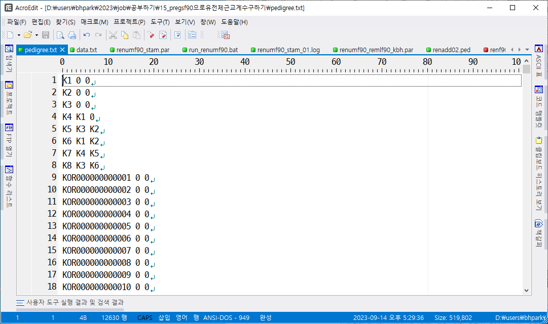
먼저 혈통 자료
animal,sire,dam
a1,0,0
a2,0,0
a3,0,0
a4,0,0
a9,0,0
a10,0,0
a11,0,0
a14,0,0
a5,a1,a2
a6,a3,a4
a7,a5,a6
a12,a9,a10
a13,a12,a11
a8,a5,a7
그림을 그려 보면 세 개의 그룹으로 이루어진 것을 알 수 있다.
R 소스
pedi <-
read.table(
"pedi_group.csv",
header = TRUE,
sep = ",",
stringsAsFactors = FALSE
)
pedi
pedi2 = cbind(pedi, flag = rep(0, nrow(pedi)), group = rep(0, nrow(pedi)))
pedi2
group_num = 0
for (i in 1:nrow(pedi2)) {
if (pedi2[i, "flag"] == 0) {
group_num = group_num + 1
temp = data.frame(animal = pedi2[i, "animal"], stringsAsFactors = FALSE)
j = 1
while (j <= nrow(temp)) {
index = which(pedi2$animal == temp[j, "animal"])
if (length(index) != 0 &&
pedi2[index, "flag"] == 0) {
pedi2[index, "flag"] = 1
pedi2[index, "group"] = group_num
sire = pedi2[index, "sire"]
if (sire != 0) {
temp = rbind(temp, sire)
}
dam = pedi2[index, "dam"]
if (dam != 0) {
temp = rbind(temp, dam)
}
index = which(pedi2$sire == temp[j, "animal"] & pedi2[which(pedi2$sire == temp[j, "animal"]), "flag"] == 0)
progeny = as.data.frame(pedi2[index, "animal"])
names(progeny) = names(temp)
temp = rbind(temp, progeny)
index = which(pedi2$dam == temp[j, "animal"] & pedi2[which(pedi2$dam == temp[j, "animal"]), "flag"] == 0)
progeny = as.data.frame(pedi2[index, "animal"])
names(progeny) = names(temp)
temp = rbind(temp, progeny)
if( (j %% 1000) == 1 ){
print(paste("Group " , group_num , ": ", j, " processing"))
}
}
j = j + 1
}
}
}
pedi2 = pedi2[order(pedi2$group), ]
pedi2
실행 결과
>
> pedi <-
+ read.table(
+ "pedi_group.csv",
+ header = TRUE,
+ sep = ",",
+ stringsAsFactors = FALSE
+ )
> pedi
animal sire dam
1 a1 0 0
2 a2 0 0
3 a3 0 0
4 a4 0 0
5 a9 0 0
6 a10 0 0
7 a11 0 0
8 a14 0 0
9 a5 a1 a2
10 a6 a3 a4
11 a7 a5 a6
12 a12 a9 a10
13 a13 a12 a11
14 a8 a5 a7
>
> pedi2 = cbind(pedi, flag = rep(0, nrow(pedi)), group = rep(0, nrow(pedi)))
> pedi2
animal sire dam flag group
1 a1 0 0 0 0
2 a2 0 0 0 0
3 a3 0 0 0 0
4 a4 0 0 0 0
5 a9 0 0 0 0
6 a10 0 0 0 0
7 a11 0 0 0 0
8 a14 0 0 0 0
9 a5 a1 a2 0 0
10 a6 a3 a4 0 0
11 a7 a5 a6 0 0
12 a12 a9 a10 0 0
13 a13 a12 a11 0 0
14 a8 a5 a7 0 0
>
> group_num = 0
>
> for (i in 1:nrow(pedi2)) {
+
+
+ if (pedi2[i, "flag"] == 0) {
+
+
+ group_num = group_num + 1
+
+
+ temp = data.frame(animal = pedi2[i, "animal"], stringsAsFactors = FALSE)
+
+
+ j = 1
+ while (j <= nrow(temp)) {
+
+
+ index = which(pedi2$animal == temp[j, "animal"])
+ if (length(index) != 0 &&
+ pedi2[index, "flag"] == 0) {
+
+ pedi2[index, "flag"] = 1
+
+
+ pedi2[index, "group"] = group_num
+
+
+ sire = pedi2[index, "sire"]
+
+
+ if (sire != 0) {
+
+ temp = rbind(temp, sire)
+ }
+
+
+ dam = pedi2[index, "dam"]
+
+
+ if (dam != 0) {
+
+ temp = rbind(temp, dam)
+ }
+
+
+ index = which(pedi2$sire == temp[j, "animal"] & pedi2[which(pedi2$sire == temp[j, "animal"]), "flag"] == 0)
+ progeny = as.data.frame(pedi2[index, "animal"])
+ names(progeny) = names(temp)
+ temp = rbind(temp, progeny)
+
+
+ index = which(pedi2$dam == temp[j, "animal"] & pedi2[which(pedi2$dam == temp[j, "animal"]), "flag"] == 0)
+ progeny = as.data.frame(pedi2[index, "animal"])
+ names(progeny) = names(temp)
+ temp = rbind(temp, progeny)
+
+
+ if( (j %% 1000) == 1 ){
+ print(paste("Group " , group_num , ": ", j, " processing"))
+ }
+
+ }
+ j = j + 1
+ }
+ }
+ }
[1] "Group 1 : 1 processing"
[1] "Group 2 : 1 processing"
[1] "Group 3 : 1 processing"
>
> pedi2 = pedi2[order(pedi2$group), ]
> pedi2
animal sire dam flag group
1 a1 0 0 1 1
2 a2 0 0 1 1
3 a3 0 0 1 1
4 a4 0 0 1 1
9 a5 a1 a2 1 1
10 a6 a3 a4 1 1
11 a7 a5 a6 1 1
14 a8 a5 a7 1 1
5 a9 0 0 1 2
6 a10 0 0 1 2
7 a11 0 0 1 2
12 a12 a9 a10 1 2
13 a13 a12 a11 1 2
8 a14 0 0 1 3
>
실제 자료일 경우 출력을 하면 안 될 것이고, 대신 head, tail, nrow 등으로 파악해야 할 것이다. 그리고 처리 중임을 표시하는 부분도 1,000개마다 할 지, 10,000개마다 할 지 수정해야 한다.