유전체 자료를 이용하여 실제 근교 계수 또는 혈연 계수를 구할 수 있다. 그러면 지금까지 혈통으로 구한 근교 계수 또는 혈연 계수는 실제가 아닌가? 그렇다. 혈통 정보에 기반하기 때문에 혈통이 없다면 또는 잘못되었다면 근교 계수 또는 혈연 계수가 0이 나오고, 혈통이 올바르다고 하여도 확률적인 근교 계수이다. 수 세대에 걸친 올바른 혈통이 있다면 확률적인 근교 계수와 실제 근교 계수의 차이가 크지 않을 것이다. 이 차이가 크다면 혈통이 올바르지 않거나 충분하지 않다고 생각할 수 있다. 여기서는 blupf90 family of programs의 하나인 pregsf90을 이용하여 유전체(실제) 근교 계수를 구해 본다. qcf90으로 구하면 좋겠지만 quality control과 근교 계수는 관계가 없는지 지금은 qcf90에서 구할 수 없다. pregsf90을 이용할 경우 renumf90 과정을 거쳐야 하고, 형식적이지만 자료 파일을 준비해야 한다는 귀찮음이 있다. 그래서 형식적인 자료로 단형질 개체 모형 예제의 자료를 이용한다.
# Parameter file for program renf90; it is translated to parameter
# file for BLUPF90 family programs.
DATAFILE
data.txt
TRAITS
3
FIELDS_PASSED TO OUTPUT
WEIGHT(S)
RESIDUAL_VARIANCE
40
EFFECT
2 cross numer
EFFECT
1 cross alpha
RANDOM
animal
FILE
pedigree.txt
FILE_POS
1 2 3
SNP_FILE
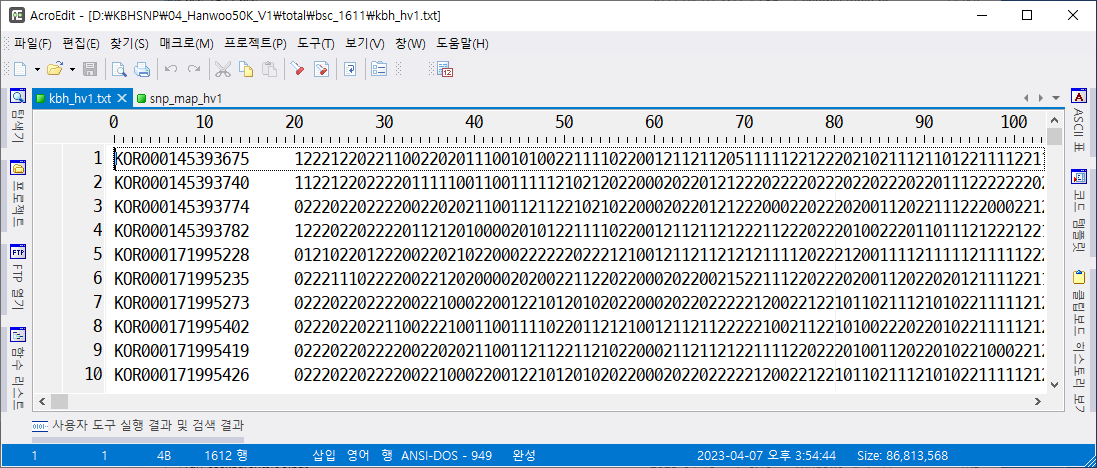
kbh_hv1.txt
PED_DEPTH
0
(CO)VARIANCES
20
snp 파일도 포함되어 있고, PED_DEPTH를 0으로 하여 혈통 파일의 모든 개체를 분석에 포함한다. 실행
renumf90 renumf90_stam.par | tee renumf90_stam_01.log
실행을 하면 여러 파일이 생긴다. renf90.par : 새로운 파라미터 파일 renf90.inb : 근교계수 renf90.dat : 리넘버된 data 파일 renf90.fields : renf90.dat에서 각 필드에 대한 설명 renadd02.ped : 리넘버된 혈통 kbh_hv1.txt_XrefID : 유전체 자료 ID의 리넘버. cross reference id 등과 같은 파일이 생긴다.
아래 세 줄을 추가한다. “OPTION methodDiagH 1” 이 부분은 “OPTION methodDiagH 2”로도 분석할 수 있다.
pregsf90 실행
SET OMP_STACKSIZE=64M
pregsf90 renf90_pregsf90.par | tee pregsf90_01.log
diagH.txt
H matrix의 대각원소만 저장한 파일이다. 전 개체에 대해서 H matrix를 만들고 그 대각원소만 추출한 것이므로 이것들 중 유전체 자료를 가진 것만 추출하고 1을 빼면 유전체 근교 계수를 구할 수 있다. OPTION methodDiagH 1을 OPTION methodDiagH 2로 변경하고 다시 실행해 보자. 실행
SET OMP_STACKSIZE=64M
pregsf90 renf90_pregsf90.par | tee pregsf90_01.log
diagHdirect.txt
개체 ID, H matrix의 대각 원소, A matrix(혈통 기반 nemerator relationship matrix)의 대각 원소, 두 대각 원소의 차이. A matrix의 대각 원소 값을 보면 혈통에 기반한 것이므로 1 또는 1.125등의 값을 보이지만, H matrix의 대각 원소는 유전체(실현) 근교 계수여서 매우 다양한 값을 볼 수 있다. 이 차이가 크다면 혈통 정보의 오류 또는 부족으로 볼 수 있다. “OPTION methodDiagH 1”와 “OPTION methodDiagH 2”의 유전체 근교 계수를 비교해 보는 것도 좋을 것이다. 두 방법의 차이는 다음을 참조한다.
G_Orig.txt 파일은 G matrix의 상삼각(또는 하삼각)을 보여준다. 이 값은 혈연 계수가 아니다. 혈연 계수는 근교 계수를 포함하여 계산한다. 하지만 근교 계수가 0이라고 가정한다면 혈연 계수라 볼 수 있다. 암튼 두 개체 사이의 관계 정도라 볼 수 있다. 혈통 정보가 부족할 경우 개체 사이의 혈연 관계 정도를 볼 수 있다. 유전체 자료는 있으나 혈통 정보가 부족한 소규모 집단의 계획 교배를 할 때 유전체 자료를 이용하여 개체의 근교 계수 또는 개체들 사이의 혈연 계수를 구하여 근친 교배를 피하고, 근교 퇴화를 예방할 수 있다.
육종을 하면서 집단에 있는 개체들의 근교계수를 계속 계산하는 것은 매우 중요한 일이다. 근친교배(inbreeding)가 일어나면 근교퇴화(inbreeding depression)가 발생하기 때문이다. 근교퇴화란 치사 유전자가 발현하여 죽어 버리거나 죽지 않더라도 경제 능력이 감소하는 현상을 말한다. 근교계수를 계산해 주는 수많은 프로그램들이 있지만 오늘은 inbupgf90을 이용하여 근교계수를 계산해 보자. inbupgf90을 다운로드 하자. http://nce.ads.uga.edu/html/projects/programs/Windows/64bit/
cd .. 명령어로 상위 폴더로 이동 cd .. 명령어로 한번 더 상위 폴더로 이동 cd blupf90으로 blupf90 폴더로 이동 dir 명령어로 폴더 내의 파일 확인
inbupgf90 명령어로 프로그램 실행
설치가 잘 된 것을 확인할 수 있다.마지막으로 모든 폴더에서 실행이 가능하도록 path를 설정하자.윈도우 시작 -> 설정 -> 정보 -> 고급 시스템 설정
환경 변수 클릭
시스템 변수 -> Path -> 편집 클릭
새로 만들기 클릭
C:\blupf90 입력하고 확인명령 프롬프트를 다시 실행하면 어떤 폴더에서든지 inbupgf90을 실행할 수 있다.
지금까지 프로그램을 실행하기 위한 환경 설정이었다. 한가지 더. D: 드라이브로 이동하기 위해서는 D: 명령어를 입력한다.
다시 기억해 보자. 위로 올라가는 명령어는 "cd .." 그리고 폴더로 이동하는 명령어는 "cd 폴더이름"이다.
이제 자료를 준비하고 프로그램을 실행하여 근교계수를 계산해 보자. 그리고 미래에 태어날 개체의 근교계수를 계산해 보자. 근교 계수를 구할 개체들의 혈통 자료 준비
여기서는 12422두를 준비하였다. 부모를 모를 경우 0으로 기입한다. 여기서 개체, 아비 및 어미 사이를 탭을 사용하여 구분하지 말고, 스페이스를 사용하여 구분한다. 엑셀에서 copy & paste를 할 경우 탭으로 구분된 경우가 있다. 이럴 경우 탭을 복사해서 찾아서 바꾸기를 할 수도 있고, 에디터에서 탭을 스페이스로 변환할 수 있다. 각자 편한 방법으로. 다음과 같은 간단한 명령어로 근교계수 계산이 끝난다.
inbupgf90 --pedfile kbh_pedi_ori_202305.txt --method 3 | tee inbupgf90_01.log
--pedfile 뒤에 혈통 파일의 이름을 적어 준다. 근교계수 계산 방법을 지정할 수 있다. 1번과 2번은 Aguilar & Misztal, 2008의 방법을 이용하고 3번은 Meuwissen & Luo 1992의 방법을 이용한다. --method 옵션을 생략하면 2번 방법을 이용하는데 메모리에서 계산하여 빠르지만 많은 메모리를 요구한다. 그러나 그렇게 많은 혈통이 있나 모르겠다. 그냥 생략해도 된다. | tee inbupgf90_01.log 는 inbupgf90_01.log 파일에 화면에 나오는 정보를 저장하고 나중에 천천히 보기 위함이다. 그런데 이 tee 명령이 실행될려면 윈도우에 프로그램을 설치해야 하는데 그건 다음 포스팅을 참조한다. 복잡하다고 느낀다면 " | tee inbupgf90_01.log" 없이 실행한다.
근교계수를 계산했는데 태어난 개체의 근교계수를 계산하면 뭐하나. 태어나기 전에 계산을 해서 근교계수가 높을 것 같으면 그런 교배를 회피해야 한다. 그래서 inbupgf90에서는 미래에 태어날 개체의 근교계수를 계산해 준다. 교배에 사용할 아비와 어미 목록을 준비하면 각각의 아비와 각각의 어미가 교배하여 태어날 개체의 근교계수를 알려준다. 먼저 교배에 사용할 아비 목록을 준비한다.
어미별로 각 아비와 교배했을 때 태어날 개체의 근교계수를 계산해 주고, 그 중 가장 근교계수를 보인 아비를 표시해 준다. 그러나 그 아비의 근교계수만 최소인 것은 아니다. 다른 아비와 교배해도 0인 경우가 많다. 보고 고르면 된다. _relationships 파일은 아비 사이의 혈연 계수를 보여준다.
마지막 열의 수는 _matings 파일에 추천 아비로 몇 번 되었는지를 나타내는 수이다. 교배계획을 어떻게 할 것인가? 근교계수가 최소로 상승하면서 최대의 능력을 발휘하는 교배가 좋은 교배이긴 하겠지만 그게 쉽지 않다. 어떤 아비가 집단의 어미와 근교도 안 되고 능력도 최고치로 올린다고 해서 모든 어미에 교배하면 그 다음 세대에 곤란한 일이 발생할 것이다. 이와 관련된 문제를 멋지게 풀어 보려고 Optimal Contribution Selection이란 개념도 생긴 거 같다. 사용 가능한 아비를 골라 보고, 어미를 기준으로 어느 정도 이하의 근교계수를 보이는 아비들을 골라보고 그 아비 중 최대의 능력을 보이는 아비를 골라보자. 그리고 전체적으로 골고루 골라졌나 보자. 한 두 개의 아비로 몰렸다면 적당히 조정하자.
유전 평가하고 상관 없으나 혈통이 있을 때 부모 또는 자식으로 연결하였을 때 몇 개의 그룹으로 나누어질지 궁금할 때가 있다. 물론 그림을 그리면 되긴 하지만, 몇십 개 이상은 그림을 그리기가 힘들다. 물론 포트란 소스로 올린 적도 있으나 컴파일하기도 힘들어서 누가 쓸까 싶다. 그래서 간단히 R로 만들어 보았다. 포트란보다 많이 느리겠지만 ...
qcf90 또는 pregsf90 프로그램을 통해서 대부분의 SNP genotype quality control을 수행할 수 있다. 그러나 이런 프로그램들은 여러 버전의 마이크로 어레이를 동시에 이용하여 quality control을 할 수 없고, 하려 한다면 imputation을 해야 한다. imputation이 필요하다면 imputation을 해서 quality control을 하면 되나, raw data를 그대로 이용하여 친자감정을 하거나 부모를 찾으려 하는 경우도 있다. seekparentf90은 약간(?)의 자료 가공을 거쳐 imputation 하지 않고, 친자 감정하거나 부모를 찾을 수 있는 기능을 제공하고 있다.
먼저 BovineSNP50V2, BovineSNP50V3, Hanwoo50V1의 GenomeStudio에서 출력한 finalreport를 illumina2pregs 프로그램을 이용하여 coded하였다고 하자. 그럴 경우 각 버전의 genotype과 map file은 다음과 같다.
BovineSNP50V2
- genotype
- map file
BovineSNP50V3
- genotype
- map file
Hanwoo50V1
- genotype
- map file
먼저 map file을 합쳐야 한다.
세 개의 map file을 읽어서 seekparentf90을 위한 map file 만드는 SAS 프로그램
/*
file name : make_snpmapfile_for_seekparentf90.sas

seekparentf90 프로그램을 위한 map file 만들기

BovineSNP50V2, BovineSNP50V3, HanwooSNP50V1 map file을 하나로 합치기
*/

/* BovineSNP50V2 snp_map 파일 읽기 */
data a1 ;
    infile 'snp_map_bv2' firstobs = 2;

    informat name $37. ;
    informat bv2chrmo best32. ;
    informat bv2pos best32. ;
    informat bv2oindex best32. ;

    format name $37. ;
    format bv2chrmo best32. ;
    format bv2pos best32. ;
    format bv2oindex best32. ;

    input
            name
            bv2chrmo
            bv2pos
            bv2oindex
    ;

    bv2index = _n_;
run;

/* BovineSNP50V3 snp_map 파일 읽기 */
data b1 ;
    infile 'snp_map_bv3' firstobs = 2;

    informat name $37. ;
    informat bv3chrmo best32. ;
    informat bv3pos best32. ;
    informat bv3oindex best32. ;

    format name $37. ;
    format bv3chrmo best32. ;
    format bv3pos best32. ;
    format bv3oindex best32. ;

    input
            name
            bv3chrmo
            bv3pos
            bv3oindex
    ;

    bv3index = _n_;
run;

/* HanwooSNP50V1 snp_map 파일 읽기 */
data c1 ;
    infile 'snp_map_hv1' firstobs = 2;

    informat name $37. ;
    informat hv1chrmo best32. ;
    informat hv1pos best32. ;
    informat hv1oindex best32. ;

    format name $37. ;
    format hv1chrmo best32. ;
    format hv1pos best32. ;
    format hv1oindex best32. ;

    input
            name
            hv1chrmo
            hv1pos
            hv1oindex
    ;

    hv1index = _n_;
run;

/* bv2, bv3, hv1 머지하기 */
    /* sort */
proc sort data = a1;
    by name;
run;

proc sort data = b1;
    by name;
run;

proc sort data = c1;
    by name;
run;

    /* 머지하기 */
data t1;
    merge a1 b1 c1;
    by name;
run;

/* 이름은 같은데 염색체, 위치가 다른 SNP */
/* 있으면 안된다. 있다면 아마도 genome build가 칩마다 다른 것일 수도 */
data t1_e1;
    set t1;

	/* bv2와 bv3 비교 */
	if bv2chrmo ~= . and bv3chrmo ~= . and bv2chrmo ~= bv3chrmo then output;

	/* bv3와 hv1 비교 */
	if bv3chrmo ~= . and hv1chrmo ~= . and bv3chrmo ~= hv1chrmo then output;
run;

/* index, 염색체 번호, 위치 번호 정리 */
data t2;
    set t1;

    /* 없었던 SNP index는 0 */
    if bv2index = . then bv2index = 0;
    if bv3index = . then bv3index = 0;
    if hv1index = . then hv1index = 0;

    /* 각 SNP의 염색체 번호 */
    chr = bv2chrmo;
    if bv2chrmo   = . then chr = bv3chrmo;
    if bv2chrmo   = . and bv3chrmo = . then chr = hv1chrmo;

    /* 각 SNP의 위치 */
    pos = bv2pos;
    if bv2pos   = . then pos = bv3pos;
    if bv2pos   = . and bv3pos = . then pos = hv1pos;

run;

/* dataset을 열어서 확인 */
proc sort data = t2;
    by chr pos;
run;

data _null_;
    set t2;
    file 'mapfile_for_seekparentf90.txt';
    if _n_ = 1 then put "SNP_ID                                  Chr       Pos       chip1     chip2     chip3";
    put name @41 chr @51 pos @61 bv2index @71 bv3index @81 hv1index;
run;
결과적으로 만들어진 map file은 다음과 같다.
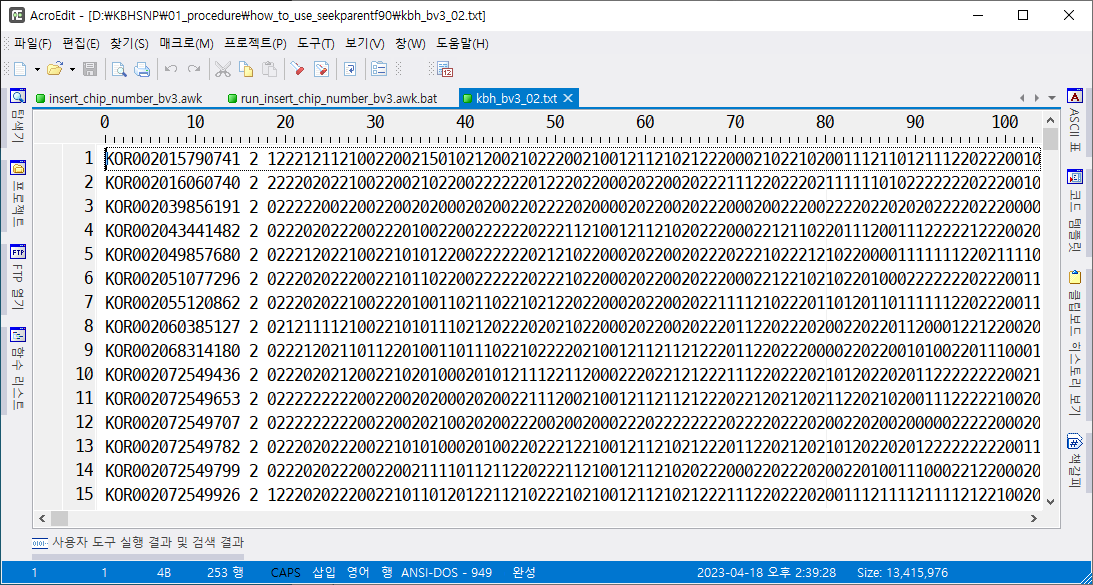
각 genotype 파일에 chip number를 넣어야 한다.
BovineSNP50V2에 chip number 1을 넣는 awk 프로그램은 다음과 같다. insert_chip_number_bv2.awk로 저장한다.
위 명령어를 run_seekparentf90.bat으로 저장하면 더블클릭으로 실행할 수 있다.
명령어 설명
seekparentf90 명령어
--pedfile kbh_pedigree_yob.txt 혈통 파일. 혈통 파일은 header 없음.
--snpfile kbh_genotype.txt 위에서 준비한 genotype 파일
--chips mapfile_for_seekparentf90.txt 위에서 준비한 map file
--yob 혈통의 넷째 컬럼에 출생연도가 있음
--seeksire_in_ped 혈통에서 아비 찾기
--seekdam_in_ped 혈통에서 어미 찾기
--exclude_chr 30 31 32 33 30에서 33번 염색체는 제외
--seektype 1 불일치인 경우만 아비 및 어미 찾기
--duplicate 유전자형이 중복인 개체들이 있는지 검사
--full_log_checks 많은 로그 기록
| tee seekparentf90_01.log 화면에 프린트되는 것을 파일에도 기록
로그는 다음과 같다.
  ----------------------------------------------------
 |                  SeekParentf90                     |
 |              Parent-Offspring tests                |
 |            and detection of paternity              |
 |               based on SNP markers                 |
 |                                                    |
 |                2013 - Version 1.47                 |
 |           (Last update:  Dec 15, 2022)             |
 |                                                    |
 |                                                    |
 |             INIA Las Brujas, Uruguay               |
 |        University of Georgia, Athens, US           |
  ----------------------------------------------------

 Options
    --pedfile kbh_pedigree_yob.txt
    --snpfile kbh_genotype.txt
    --yob
    --seeksire_in_ped
    --seekdam_in_ped
    --seektype 1
    --chips mapfile_for_seekparentf90.txt
    --exclude_chr 30 31 32 33
    --full_log_checks

 Using Jenkins hash function

 Maximum length for alphanumeric fields: 20

 Fields to read:  animal, sire, dam, yob (4)

 Elapsed time for reading and hash: .250

 Pedigree file "kbh_pedigree_yob.txt": 12412 records

 Total number of animals in pedigre: 12412

 Statistics for Year of Birth
  Minimun:         1990
  Maximun:         2023

 Read multiple Chip SNP file: "kbh_genotype.txt"

 Number of SNP from snp_info file: 60961

 ***** WARNING *****  Number of duplicate SNP by chr_pos: 93
 ***** List of duplicate SNP: "duplicate_snp_chr_pos"

 Exclude Chr(s)
   Chr:  30  1190
   Chr:  31    11
   Chr:  32    13
   Chr:  33   775

 Chip identification
   Chip   1: CHIP1
   Chip   2: CHIP2
   Chip   3: CHIP3


 Number of SNP by Chip
   Chip   1:    54609   50908   47514
   Chip   2:        0   53218   49760
   Chip   3:        0       0   53866

 Exclude SNP: 1989
 Maximum Available SNP for calculations: 58972


 Number of effective SNP by Chip for parent-progeny conflicts
   Chip   1:    52886   49233   46109
   Chip   2:        0   51278   48090
   Chip   3:        0       0   52195
    Column position in file for the first marker: 19
    Format to read SNP file: (18x,800000i1)
    Number of SNPs: 60961

 Threshold for exclusions - Maximun number of SNP: 58972
 Number of SNP > 130, set the threshold probability to exclude= 1.000
 Number of SNP > 130, set the threshold probability to assign = .500
 Threshold based on percent of conflicts to exclude: 1.000
 Threshold based on percent of conflicts to assign: .500

 Number of records in SNP file: 1884
 Number of records present in pedigree: 1883 1883

 Number of records by Chip
    Chip 1: 21
    Chip 2: 252
    Chip 3: 1611

 Call Rate
   Min CR:   5346 .90
   Max CR:     42 1.00
   AVG CR:    668 .99
   Number of samples with low call rate (  0.90 ):      0

 Samples with low call rate for effective SNP           0

 Check all pedigree for parent-progeny conflicts

 Pedigree records with genotype: 1883

 Records not tested (low call rate <  0.90 ): 0

 Records tested: 1883

 Pair parent/progeny tested: 1403
 Pair with conflicts: 19   1.4 %
   NOT tested (parent low call rate): 0

     Sire-progeny tested: 715
     Sire-progeny with conflicts: 11   1.5 %
       NOT tested (parent low call rate): 0

     Dam-progeny tested: 688
     Dam-progeny with conflicts: 8   1.2 %
       NOT tested (parent low call rate): 0

 Seek parent for SIRES
   Get list of parents: detected from pedigree
     Number of Sires: 171

   Seek method: Only for animals with conflicts

   Total number of animals: 11
      Found: 7
      Not Found: 4
      Found but cannot assign: 0

 Seek parent for DAMS
   Get list of parents: detected from pedigree
     Number of Dams : 666

   Seek method: Only for animals with conflicts

   Total number of animals: 8
      Found: 3
      Not Found: 5
      Found but cannot assign: 0

 Output files
     Pedigree file with removed parents for animals with conflicts: "Check_kbh_pedigree_yob.txt"

 Full reports
     "Parent_Progeny_Conflicts.txt"
     "Parent_Progeny_Conflicts_Summary.txt"
     "Seek_Sire.txt"
     "Seek_Dam.txt"
중간에
***** WARNING ***** Number of duplicate SNP by chr_pos: 93
***** List of duplicate SNP: "duplicate_snp_chr_pos“
로그가 있는데 duplicate_snp_chr_pos 파일을 열어 보면 다음과 같다,
Duplicate SNP chr_pos: 1_59409838 2
Duplicate SNP chr_pos: 13_25606469 2
Duplicate SNP chr_pos: 3_58040470 2
Duplicate SNP chr_pos: 14_27271835 2
Duplicate SNP chr_pos: 29_28647816 2
Duplicate SNP chr_pos: 15_15014275 2
Duplicate SNP chr_pos: 2_50689222 2
Duplicate SNP chr_pos: 11_33265117 2
Duplicate SNP chr_pos: 7_1071389 2
Duplicate SNP chr_pos: 15_79531511 2
Duplicate SNP chr_pos: 9_45729853 2
Duplicate SNP chr_pos: 25_10359385 2
Duplicate SNP chr_pos: 22_56526462 2
Duplicate SNP chr_pos: 20_676757 2
Duplicate SNP chr_pos: 22_8308367 2
Duplicate SNP chr_pos: 20_17837675 2
Duplicate SNP chr_pos: 14_56761589 2
Duplicate SNP chr_pos: 3_76797698 2
Duplicate SNP chr_pos: 25_26191380 2
Duplicate SNP chr_pos: 19_43264699 2
Duplicate SNP chr_pos: 21_65198296 2
Duplicate SNP chr_pos: 8_106174871 2
Duplicate SNP chr_pos: 15_15367990 2
Duplicate SNP chr_pos: 2_111155237 2
Duplicate SNP chr_pos: 14_76524093 2
Duplicate SNP chr_pos: 13_71212300 2
Duplicate SNP chr_pos: 14_25401722 2
Duplicate SNP chr_pos: 12_80629629 2
Duplicate SNP chr_pos: 10_49791638 2
Duplicate SNP chr_pos: 6_54524018 2
Duplicate SNP chr_pos: 3_40654331 2
Duplicate SNP chr_pos: 15_15595454 2
Duplicate SNP chr_pos: 7_21298998 2
Duplicate SNP chr_pos: 15_15738972 2
Duplicate SNP chr_pos: 7_18454636 2
Duplicate SNP chr_pos: 7_80042191 2
Duplicate SNP chr_pos: 26_38233337 2
Duplicate SNP chr_pos: 28_35331560 2
Duplicate SNP chr_pos: 15_77675440 2
Duplicate SNP chr_pos: 15_15908105 2
Duplicate SNP chr_pos: 26_8221270 2
Duplicate SNP chr_pos: 18_1839733 2
Duplicate SNP chr_pos: 15_15697628 2
Duplicate SNP chr_pos: 11_1703612 2
Duplicate SNP chr_pos: 15_21207529 2
Duplicate SNP chr_pos: 15_79187295 2
Duplicate SNP chr_pos: 22_31841994 2
Duplicate SNP chr_pos: 20_51449833 2
Duplicate SNP chr_pos: 15_15544958 2
Duplicate SNP chr_pos: 15_15520367 2
Duplicate SNP chr_pos: 15_15656347 2
Duplicate SNP chr_pos: 15_15305071 2
Duplicate SNP chr_pos: 6_61079420 2
Duplicate SNP chr_pos: 15_15213319 2
Duplicate SNP chr_pos: 16_38116988 2
Duplicate SNP chr_pos: 28_44261945 2
Duplicate SNP chr_pos: 9_10783460 2
Duplicate SNP chr_pos: 14_48380429 2
Duplicate SNP chr_pos: 29_13695183 2
Duplicate SNP chr_pos: 1_136603695 2
Duplicate SNP chr_pos: 15_15162470 2
Duplicate SNP chr_pos: 15_15245842 2
Duplicate SNP chr_pos: 3_116448759 2
Duplicate SNP chr_pos: 15_38078775 2
Duplicate SNP chr_pos: 15_15190242 2
Duplicate SNP chr_pos: 8_95410507 2
Duplicate SNP chr_pos: 3_91910014 2
Duplicate SNP chr_pos: 17_60069612 2
Duplicate SNP chr_pos: 9_98483346 2
Duplicate SNP chr_pos: 12_79289169 2
Duplicate SNP chr_pos: 1_151349514 2
Duplicate SNP chr_pos: 4_17200594 2
Duplicate SNP chr_pos: 19_47734925 2
Duplicate SNP chr_pos: 26_47781927 2
Duplicate SNP chr_pos: 8_88974063 2
Duplicate SNP chr_pos: 14_29987025 2
Duplicate SNP chr_pos: 14_31322421 2
Duplicate SNP chr_pos: 14_21343649 2
Duplicate SNP chr_pos: 1_1277227 2
Duplicate SNP chr_pos: 24_4118163 2
Duplicate SNP chr_pos: 13_49053256 2
Duplicate SNP chr_pos: 10_55611885 2
Duplicate SNP chr_pos: 28_8508619 2
Duplicate SNP chr_pos: 6_55756520 2
Duplicate SNP chr_pos: 15_15949175 2
Duplicate SNP chr_pos: 4_94176209 2
Duplicate SNP chr_pos: 14_23893220 2
Duplicate SNP chr_pos: 25_26198573 2
Duplicate SNP chr_pos: 16_33671664 2
Duplicate SNP chr_pos: 3_71860062 2
Duplicate SNP chr_pos: 5_63150400 2
Duplicate SNP chr_pos: 7_37537822 2
Duplicate SNP chr_pos: 9_32549297 2
93개의 염색체 번호와 위치에서 염색체 번호와 위치는 같은데 서로 다른 SNP 이름을 갖고 있다는 에러를 뿌려줌. 유전체 선발에서는 제외를 하겠지만 여기서는 제외를 해야 올바른 것인지 잘 모르겠다. 분석에서 93쌍 즉 186개 SNP를 이용했는지 안 했는지 모르겠다.
Pair parent/progeny tested: 1403
Pair with conflicts: 19 1.4 %
1403개 부모/자식을 테스트해서 19개 관계가 친자감정 불일치
Sire-progeny tested: 715
Sire-progeny with conflicts: 11 1.5 %
715개 아비/자식을 테스트해서 11개 관계가 불일치
Dam-progeny tested: 688
Dam-progeny with conflicts: 8 1.2 %
688개 어미/자식을 테스트해서 8개 관계가 불일치
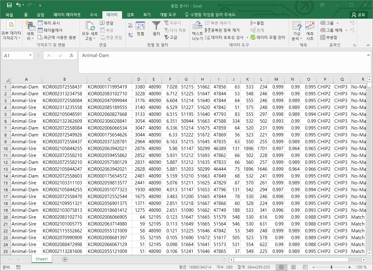
parent_progeny_conflicts.txt
개체와 부모의 친자감정 결과를 보여준다. 그러나 너무 자세해서 보기 어렵다.
정렬을 해서 animal-dam 그리고 animal-sire 부분을 엑셀로 복사하고, D열을 내림차순 정렬하면 친자감정 불일치 개체 19두를 찾을 수 있다.
친자감정 불일치가 일어나는 경우는 세 가지이다. 1) 부(모)의 유전자형이 잘못 되었다. 2) 자손의 유전자형이 잘못되었다. 3) 혈통이 잘못되었다.
친자감정 불일치가 일어날 경우 1)과 2)를 생각안하고 무턱대고 3)을 생각할 경우 심각한 문제를 초래할 수 있다. 그러면 유전자형이 정말 제대로 되었는지는 어떻게 알 수 있는가?
parent_progeny_conflicts_summary.txt를 보자.
KOR002085189555 개체의 경우는 아비로서 9번 친자감정을 했고 그중 1번만 불일치다. 그러면 8번은 맞은 경우이므로 자기 자신의 유전자형이라고 확신할 수 있다.
그러나 KOR002072558437 는 개체로서 2번 친자감정 되었는데 2번다 친자감정 불일치가 났다. 이런 경우 자신의 유전자형이라고 보기 매우 힘들다. (아니라는 확신은 못한다.) 다시 genotyping을 할 수 있다면 하고, 다른 친자감정 결과 예를 들어 Microsatellite 친자감정 결과가 있다면 참고하여 결정하여야 한다.
조직을 샘플링할 때, 실험할 때, 결과를 처리할 때 등등 자신의 유전자형이 아닐 확률은 너무나 많다. 위와 같이 친자감정 일치가 하나라도 나왔다면 자신의 유전자형이라고 확신할 수 있지만 친자감정 일치가 없다면 자신의 유전자형인지 강한 의심을 하고, 그다음으로 혈통을 고민해야 한다.
A라는 개체가 B의 유전자형을 들고 우수한 개체로 판명이 나고, 그 결과를 이용하여 부모로 자손을 생산한다면 얼마나 큰 실수인가.
아래는 자신의 유전자형을 확신할 때 보는 부분이다. 즉 자신의 유전자형이 맞으므로 혈통을 수정해야 할 경우 보는 부분이다.
Seek method: Only for animals with conflicts
Total number of animals: 11
Found: 7
Not Found: 4
Found but cannot assign: 0
아비 불일치 11개 중 7개를 찾았다.
Seek method: Only for animals with conflicts
Total number of animals: 8
Found: 3
Not Found: 5
어미 불일치 8개 중 3개를 찾고, 5개는 찾지 못했다.
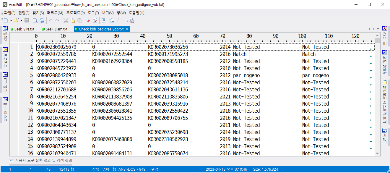
Output files
Pedigree file with removed parents for animals with conflicts: "Check_kbh_pedigree_yob.txt“
불일치인 개체의 부 또는 모 정보를 제거한 혈통 파일
아비 찾기 결과 seek_sire.txt
위에선 7개의 아비를 찾았다고 했으나 8개를 찾은 결과가 나옴. 이건 뭐지?
seek_dam.txt
3개의 어미를 찾았다.
SNP 정보를 기반으로 아비와 어미를 찾아주었다고 하여 무조건 믿는 것도 안된다. 같은 농장인지, 같은 농장이 아니라면 인공수정이나 수정란 이식인지, 부모의 나이가 많은지 등등을 종합적으로 살펴보고 수정하여야 한다.
이렇게 자기 자신의 올바른 유전자형과 올바른 혈통이 있다면 imputation 정확도가 매우 높아진다.
요약
1) 파일 준비 * genotype file - kbh_bv2.txt - kbh_bv3.txt - kbh_hv1.txt
* chip 번호 넣는 awk 파일과 awk을 실행시키는 batch 파일 - insert_chip_number_bv2.awk, run_insert_chip_number_bv2.awk.bat - insert_chip_number_bv3.awk, run_insert_chip_number_bv3.awk.bat - insert_chip_number_hv1.awk, run_insert_chip_number_hv1.awk.bat
* chip 번호 넣은 genotype file을 합치는 파일 - make_one_genotype_file.bat
주어지는 자료는 6열까지이다. fullsib 효과야 2열과 3열을 붙이면 되는 거니까 어렵지 않다. 문제는 동기축을 자료로 붙이는 일이다. 그리고 리넘된 자료로 해야 하므로 renumf90을 적당히 돌리고, 같은 펜에 있는 동기축의 renumber된 번호를 붙여야 한다. 여기서는 일단 수동으로 자료를 준비하여 분석한다.
sex 효과, direct genetic 효과는 일반적이다. 그러나 associative genetic 효과의 design matrix는 일반적인 design matrix와는 다르다. 일반적인 design matrix는 한 행에 1이 하나만 들어가나, associative genetic 효과의 design matrix는 한 행에 같은 pen(group)에 있는 동기축들을 1로 해야 한다. 그래서 7열은 레벨을 만들지 말고, 8열로만 레벨을 만들어 한 효과로 처리하고 동기축을 1로 한다는 의미이다.
실행화면
blupf90 blupf90_social.par | tee blupf90_social_01.log
로그
blupf90_social.par
     BLUPF90 ver. 1.68

 Parameter file:             blupf90_social.par
 Data file:                  social2_data.txt
 Number of Traits             1
 Number of Effects            6
 Position of Observations      6
 Position of Weight (1)        0
 Value of Missing Trait/Observation           0

EFFECTS
 #  type                position (2)        levels   [positions for nested]
    1  cross-classified       5         2
    2  cross-classified       1        15
    3  cross-classified       7         0
    4  cross-classified       8        15
    5  cross-classified       9         3
    6  cross-classified       4         3

 Residual (co)variance Matrix
  48.480

 correlated random effects     2  3
 Type of Random Effect:      additive animal
 Pedigree File:              social_pedi.txt
 trait   effect    (CO)VARIANCES
  1       2     25.70       2.250
  1       3     2.250       3.600

 Random Effect(s)    5
 Type of Random Effect:      diagonal
 trait   effect    (CO)VARIANCES
  1       5     12.50

 Random Effect(s)    6
 Type of Random Effect:      diagonal
 trait   effect    (CO)VARIANCES
  1       6     12.12

 REMARKS
  (1) Weight position 0 means no weights utilized
  (2) Effect positions of 0 for some effects and traits means that such
      effects are missing for specified traits


 * The limited number of OpenMP threads = 4

 * solving method (default=PCG):FSPAK

 Data record length =            9
 # equations =           38
 G
  25.700      2.2500
  2.2500      3.6000
 G
  12.500
 G
  12.120
 read            9  records in   0.1406250      s,                     139
  nonzeroes
  read           15  additive pedigrees
 finished peds in   0.1406250      s,                     250  nonzeroes
 solutions stored in file: "solutions"
여기서는 associative effect 는 없고, sex, animal, pen, common environment effect(full-sib) 효과만 있는 것으로 한다.
# Parameter file for program renf90; it is translated to parameter
# file for BLUPF90 family programs.
COMBINE 7 2 3
DATAFILE
social1_data.txt
TRAITS
6
FIELDS_PASSED TO OUTPUT

WEIGHT(S)

RESIDUAL_VARIANCE
48.48
EFFECT
5 cross numer
EFFECT
1 cross alpha
RANDOM
animal
FILE
social1_pedi.txt
FILE_POS
1 2 3
PED_DEPTH
0
(CO)VARIANCES
25.7
EFFECT
4 cross numer
RANDOM
diagonal
(CO)VARIANCES
12.12
EFFECT
7 cross alpha
RANDOM
diagonal
(CO)VARIANCES
12.5
OPTION sol se
 Effect group 1 of column 1 with 2 levels, effect # 1
 Value    #    consecutive number
1 4 1
2 5 2
 Effect group 3 of column 1 with 3 levels, effect # 3
 Value    #    consecutive number
1 3 1
2 3 2
3 3 3
 Effect group 4 of column 1 with 3 levels, effect # 4
 Value    #    consecutive number
a1a4 3 1
a2a5 3 2
a3a6 3 3