PostGSF90을 이용한 GWAS
PostGSF90 프로그램을 이용하여 GWAS를 할 수 있다. 먼저 각 SNP의 가중치를 1로 주어 ssGBLUP을 하고, 결과로 나온 유전체 육종가로부터 SNP marker effect와 각 SNP의 가중치를 계산한다. 이 가중치를 이용하여 ssGBLUP을 다시 실행하고, 결과로 나온 유전체 육종가로부터 SNP marker effect를 계산하여 GWAS를 한다. 이 반복을 2회 또는 3회 할 경우 결과가 바람직한 것으로 나와 있다. 그리고 현재 PostGSF90은 single trait에 대해서만 가능하다.
먼저 renumf90으로 만든 파라미터 파일을 복사하고, renf90_blupf90.par로 파일명을 바꾼다. 이미 Genomic Library를 이용하여 QC를 하였으므로 QC된 파일을 이용하여 옵션을 작성한다. 다음 옵션을 추가한다.
OPTION SNP_file 50k_for_gs.txt_clean
OPTION chrinfo snp_map_for_gs.txt_clean
OPTION no_quality_control
OPTION saveGInverse
OPTION saveA22Inverse
OPTION weightedG w
각 옵션에 대한 설명은 다음과 같다.
OPTION SNP_file 50k_for_gs.txt_clean
-> QC된 SNP
OPTION chrinfo snp_map_for_gs.txt_clean
-> QC된 SNP의 map file
OPTION no_quality_control
-> QC를 하지 않음
OPTION saveGInverse
-> GInverse를 저장
OPTION saveA22Inverse
-> A22 Inverse를 저장
OPTION weightedG w
-> 각 SNP의 가중치. 처음에는 모두 1을 줄 것임
다음 awk 명령어를 이용하여 1이 42561행(the number of SNP) 있는 w 파일을 만들 수 있다.
|
awk "BEGIN { for (i == 1 ; i < 42561 ; i++) print 1}" > w |

blupf90 실행을 위한 파라미터 파일은 다음과 같다.

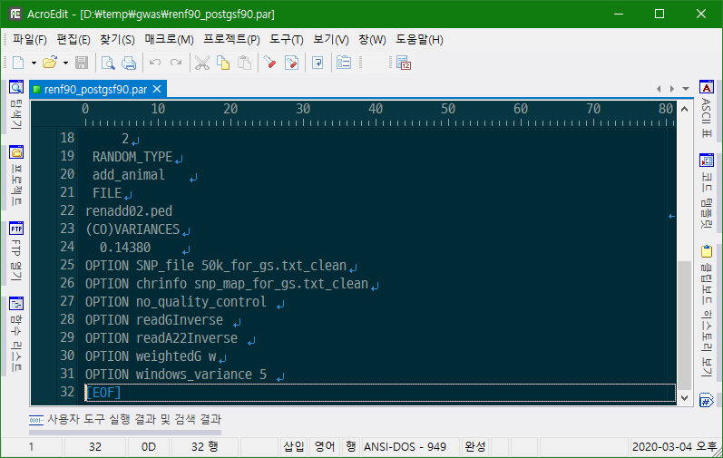
그리고 postgsf90을 실행하기 위하여 renumf90이 만든 파라미터 파일 renf90.par를 복사하고 이름을 renf90_postgsf90.par로 만든다. 다음 옵션을 추가한다.
OPTION SNP_file 50k_for_gs.txt_clean
OPTION chrinfo snp_map_for_gs.txt_clean
OPTION no_quality_control
OPTION readGInverse
OPTION readA22Inverse
OPTION weightedG w
OPTION windows_variance 5
설명은 다음과 같다.
OPTION SNP_file 50k_for_gs.txt_clean
-> QC된 SNP 사용
OPTION chrinfo snp_map_for_gs.txt_clean
-> QC된 SNP의 map file
OPTION no_quality_control
-> QC를 하지 않음
OPTION readGInverse
-> GInverse를 읽을 것
OPTION readA22Inverse
-> A22 Inverse를 읽을 것
OPTION weightedG w
-> 각 SNP 가중치 파일을 읽을 것
OPTION windows_variance 5
-> 5개의 인접한 SNP에 의하여 설명되는 분산
blupf90에서 사용하는 옵션을 지우고, postgsf90에서 필요한 옵션을 넣은 파라미터 파일을 다음과 같다.
프로그램 실행순서는 다음과 같다.
(1 라운드)
1) 각 SNP의 가중치를 1로 blupf90 실행
2) blupf90의 실행 결과인 solutions를 solutions_01로 복사
3) postgsf90 실행
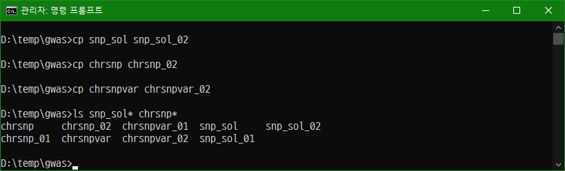
4) postgsf90 실행 결과인 snp_sol, chrsnp, chrsnpvar을 snp_sol_01, chrsnp_01, chrsnpvar_01로 복사
5) w를 w_01로 복사
6) snp_sol에서 7열을 새로운 w로 저장
|
awk “(NR > 1) {print $7}” snp_sol > w |
(2 라운드)
1) 새로운 SNP의 가중치로 blupf90 실행
2) blupf90의 실행 결과인 solutions를 solutions_02로 복사
3) postgsf90 실행
4) postgsf90 실행 결과인 snp_sol, chrsnp, chrsnpvar을 snp_sol_02, chrsnp_02, chrsnpvar_02로 복사
5) w를 w_02로 복사
6) snp_sol에서 7열을 새로운 w로 저장
|
awk “(NR > 1) {print $7}” snp_sol > w |
(3라운드) : 필요시 3라운드 실행
1 라운드를 실행하는 명령어 및 실행화면은 다음과 같다.
1) 각 SNP의 가중치를 1로 blupf90 실행
-> blupf90 renf90_blupf90.par | tee blupf90_01.log

실행 결과 생긴 파일들

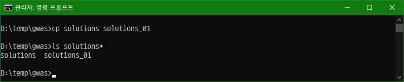
2) blupf90의 실행 결과인 solutions를 solutions_01로 복사
-> cp solutions solutions_01
3) postgsf90 실행
-> postgsf90 renf90_postgsf90.par | tee postgsf90_01.log

실행결과 생긴 파일들

4) postgsf90 실행 결과인 snp_sol, chrsnp, chrsnpvar을 snp_sol_01, chrsnp_01, chrsnpvar_01로 복사
-> cp snp_sol snp_sol_01
-> cp chrsnp chrsnp_01
-> cp chrsnpvar chrsnpvar_01


5) w를 w_01로 복사
-> cp w w_01

6) snp_sol에서 7열을 새로운 w로 저장
-> awk "(NR > 1) { print $7 }" snp_sol > w

1 라운드 끝.
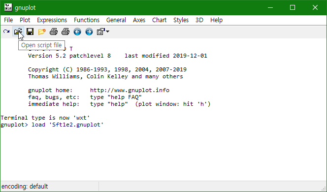
Sft1e2.gnuplot, Sft1e2.R, Vft1e2.gnuplot, Vft1e2.R은 Manhatton plot을 그리기 위한 스크립트 파일이다. S로 시작하는 파일을 SNP의 값으로 Manhatton plot을 그리기 위한 스크립트 파일이고, V로 시작하는 파일은 SNP의 분산으로 Manhatton plot을 그리기 위한 스크립트 파일이다. 확장자가 gnuplot인 것은 gnuplot 프로그램을 이용하고, 확장자가 R인 것은 R 프로그램을 이용한다.
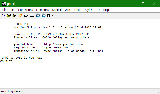
gnuplot을 실행한다.
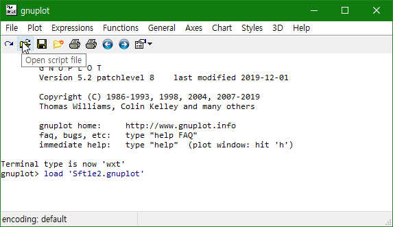
open script file을 클릭하여 Sft1e2.gnuplot을 로드한다.
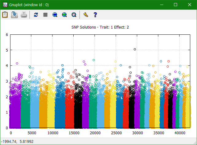
export plot to file 버튼을 눌러 plot_snp_01.png로 저장한다.
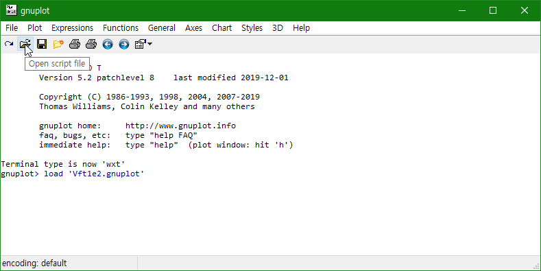
open script file을 클릭하여 Vft1e2.gnuplot을 로드한다.


export plot to file 버튼을 눌러 plot_snpvar_01.png로 저장한다.
(2 라운드)
1) 새로운 SNP의 가중치로 blupf90 실행
-> blupf90 renf90_blupf90.par | tee blupf90_02.log

2) blupf90의 실행 결과인 solutions를 solutions_02로 복사
-> cp solutions solutions_02

3) postgsf90 실행
-> postgsf90 renf90_postgsf90.par | tee postgsf90_02.log

4) postgsf90 실행 결과인 snp_sol, chrsnp, chrsnpvar을 snp_sol_02, chrsnp_02, chrsnpvar_02로 복사
-> cp snp_sol snp_sol_02
-> cp chrsnp chrsnp_02
-> cp chrsnpvar chrsnpvar_02
5) w를 w_02로 복사
-> cp w w_02

6) snp_sol에서 7열을 새로운 w로 저장
-> awk "(NR > 1) { print $7 }" snp_sol > w

gnuplot을 실행시키고 open script file을 클릭하여 Sft1e2.gnuplot을 로드한다.

export plot to file 버튼을 눌러 plot_snp_02.png로 저장한다.
open script file을 클릭하여 Vft1e2.gnuplot을 로드한다.

export plot to file 버튼을 눌러 plot_snpvar_02.png로 저장한다.
명령어만 모아 놓으면 다음과 같다.
blupf90 renf90_blupf90.par | tee blupf90_01.log
cp solutions solutions_01
postgsf90 renf90_postgsf90.par | tee postgsf90_01.log
cp snp_sol snp_sol_01
cp chrsnp chrsnp_01
cp chrsnpvar chrsnpvar_01
cp w w_01
awk "(NR > 1) { print $7 }" snp_sol > w
blupf90 renf90_blupf90.par | tee blupf90_02.log
cp solutions solutions_02
postgsf90 renf90_postgsf90.par | tee postgsf90_02.log
cp snp_sol snp_sol_02
cp chrsnp chrsnp_02
cp chrsnpvar chrsnpvar_02
cp w w_02
awk "(NR > 1) { print $7 }" snp_sol > w
윈도우즈에서 batch 파일이나, 유닉스에서 shell script를 만들 때 유용하다.
snp_sol 파일에는 다음과 같은 정보가 들어 있다.
1: trait
2: effect
3: SNP
4: Chromosome
5: Position
6: SNP solution
7: weight
if OPTION windows_variance is used
8: variance explained by n adjacents SNP.
if OPTION snp_p_value is used
9: variance of the SNP solution (used to compute the p-value)

chrsnp에는 SNP 효과의 값을 plot 하기 위한 정보가 들어 있다.
1: trait
2: effect
3: values of SNP effects to use in Manhattan plots
4: SNP
5: Chromosome
6: Position

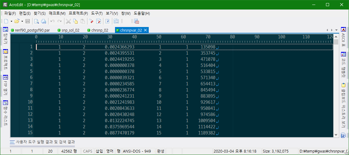
chrsnpvar에는 N개의 근접한 SNP들에 의해서 설명되는 분산을 plot 하기 위한 정보가 들어 있다.
1: trait
2: effect
3: variance explained by n adjacents SNP
4: SNP
5: Chromosome
6: Position
OPTION snp_p_value 옵션을 사용하면 SNP 효과에 대한 p-value를 구할 수 있다.
snp_sol, chrsnp 또는 chrsnpvar 파일을 이용하여 해당 형질에 major effect를 가지고 있는 SNP를 선발할 수 있다.
'Animal Breeding > Genomic Selection' 카테고리의 다른 글
| H 행렬, H 행렬의 역행렬 유도 (0) | 2021.01.19 |
|---|---|
| SNP Effect를 이용한 DGV(or GEBV) 추정 (0) | 2020.03.05 |
| SNP Marker Effect 추정 (0) | 2020.03.02 |
| blupf90을 이용하여 유전체 육종가 구하기 (0) | 2020.02.13 |
| SNP 유전체 자료를 이용한 아비 어미 찾기 (0) | 2020.02.12 |