유전체 육종가를 구하는 방법은 두 가지가 있다. 먼저 SNP 유전자형 분석을 마친 개체들의 표현형 자료를 이용하여 각 SNP 들의 효과를 구하고, 그걸 이용해서 개체의 유전체 육종가를 구하는 방법이 있다. 이 방법을 이용하면 기존의 유전체 자료를 가지고 있지 않은 개체들의 표현형 자료들이 쓸 모 없어진다. 그리고 많은 나라들이 그동안 육종가를 구하기 위하여 만든 수많은 프로그램도 동시에 쓸 모 없어진다. 그래서 기존의 표현형 자료도 살리고, 프로그램도 살리는 방법으로 개발된 것이 Single Step GBLUP이다. ssGBLUP에서는 기존의 혈통 자료와 표현형 자료를 이용한 유전능력 평가 프로세스에서 혈연 계수 행렬(Numerator Relationship Matrix, NRM)을 만들 때, SNP 유전체를 가지고 있는 개체들은 유전체 자료를 이용해서 개체들 사이의 관계를 확률적으로 구하는 것이 아니라 SNP 유전체 자료를 이용하여 실제 관계(GRM : Genomic Relationship Matrix)를 구하고, 해당 개체의 NRM을 부분을 대체하게 된다. 이렇게 만들어진 행렬을 H 행렬이라고 한다. 물론 GRM을 구하는 다양한 방법이 있으며 각각의 축종, 형질에 따라서 알맞은 GRM을 사용할 것을 권한다. 알맞은 GRM의 기준은 육종가의 정확도 등과 같은 것이 있다. 여기서는 고정효과로 전체 평균 1개만 있는, 단형질 개체 모형(single trait animal model)을 이용하여 유전체 육종가 구하는 것을 설명한다. 프로그램은 blupf90을 이용한다.
준비한 혈통은 다음과 같다.

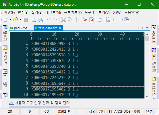
준비한 자료는 다음과 같다.
준비한 유전체 자료는 다음과 같다.

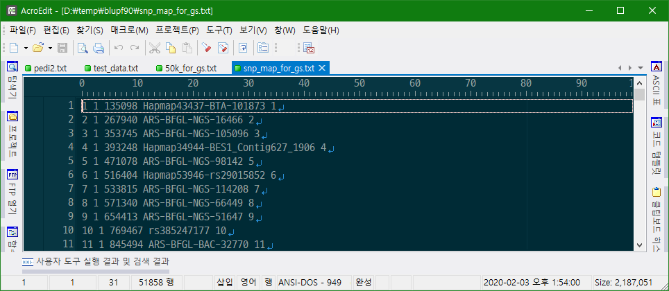
준비한 SNP map 파일은 다음과 같다.
blupf90 프로그램을 실행하기 전에 renumf90 프로그램을 실행하여 고정 효과 및 임의 효과를 renumber한다. renumf90을 실행하기 위한 파라미터 파일은 다음과 같다.
|
# single trait animal model DATAFILE test_data.txt TRAITS 2 FIELDS_PASSED TO OUTPUT
WEIGHT(S)
RESIDUAL_VARIANCE 0.6280 EFFECT 3 cross numer EFFECT 1 cross alpha RANDOM animal FILE pedi2.txt FILE_POS 1 2 3 SNP_FILE 50k_for_gs.txt PED_DEPTH 50 (CO)VARIANCES 0.1438 OPTION sol se
|
DATAFILE
test_data.txt
=> 자료 파일의 이름
TRAITS
2
=> 둘째 열이 형질
RESIDUAL_VARIANCE
0.6280
잔차의 분산
EFFECT
3 cross numer
=> 고정효과는 3열
EFFECT
1 cross alpha
RANDOM
animal
FILE
pedi2.txt
FILE_POS
1 2 3
SNP_FILE
50k_for_gs.txt
PED_DEPTH
50
(CO)VARIANCES
0.1438
=> 1열은 개체 효과인데 혈통파일의 이름은 pedi2.txt이고, 혈통 파일에 있는 열은 animal, sire, dam이고, 관련 SNP 파일은 50k_for_gs.txt이다. 혈통은 위로 50세대까지 추적하고 임의효과인 개체효과의 분산은 0.1438이다.
OPTION sol se
=> 육종가의 표준오차까지 구한다.
기타 필요한 옵션을 추가한다.
renumf90 실행명령어와 실행화면은 다음과 같다.
|
renumf90 renumf90_stam.par | tee renumf90_stam_01.log |


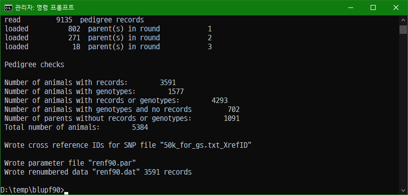
renumf90을 실행하여 생긴 파일은 다음과 같다.
renadd02.ped

혈통 파일의 개체 번호를 renumber한 것이다. 위의 파일 이름에서 02는 고정효과 및 임의효과가 2개 있다는 의미이다.
50k_for_gs.txt_XrefID

50k_for_gs.txt에 있는 개체들이 몇 번으로 renumber되었는지 나와 있다.
renf90.tables
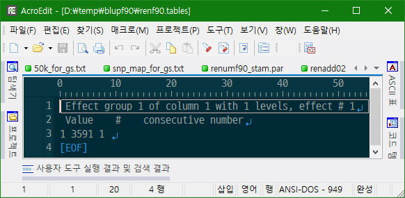
고정효과의 레벨들이 몇 번으로 renumber되었는지 나와 있다.
renf90.dat

각 효과들이 renumber되고 위치가 형질, 고정효과, 개체효과 순으로 재배열 된 것을 볼 수 있다.
renf90.par
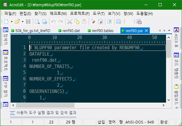
renumber된 자료를 remlf90 또는 blupf90에서 실행할 때 필요한 파라미터 파일이다.
renf90.par 파일을 복사하고 renf90_gs.par 로 이름을 바꾸고 파일의 마지막에 다음을 추가한다.
OPTION chrinfo snp_map_for_gs.txt
OPTION excludeCHR 30 31 32
OPTION saveCleanSNPs
OPTION verify_parentage 3
OPTION callrateAnim 0.90
OPTION outcallrate
OPTION outparent_progeny
설명은 다음과 같다.
OPTION chrinfo snp_map_for_gs.txt
=> SNP 맵 파일 지정
=> chrinfo 옵션은 DEPRECATED OPTIONS(곧 사라질 옵션)으로 되어 있다. 대신 map_file 옵션이 있다. 그런데 두 옵션에서 지정하는 map file의 순서가 다른다. chrinfo에서는 snp order , chromosome, position (bp)이고, map_file에서는 SNP_ID, CHR, POS이다. 그런데 illumina2pregs에서는 snp order , chromosome, position 순서의 map file을 출력하고 있다.
OPTION excludeCHR 30 31 32
=> 제외할 chromosomes
OPTION saveCleanSNPs
=> 제외할 SNP와 개체를 제거하고 SNP 유전자형 파일을 저장한다. 네 개의 파일이 생긴다.
gt_clean : 제외할 SNP와 개체를 제거한 SNP 유전자형 파일
gt_clean_XrefID : gt_clean에 있는 개체들의 renumber된 ID
gt_SNPs_removed : 제거한 SNP
gt_Animals_removed : 제거한 개체
OPTION verify_parentage 3
=> 친자감정을 하는데 conflicts가 나는 자손을 제거한다.
OPTION callrateAnim 0.90
=> call rate가 낮은 개체는 무시한다.
OPTION outcallrate
=> SNP 별로, 개체별로 call rate 정보를 출력한다. SNP에 대해서는 callrate이라는 파일이 생기고, 개체에 대해서는 callrate_a 파일이 생긴다.
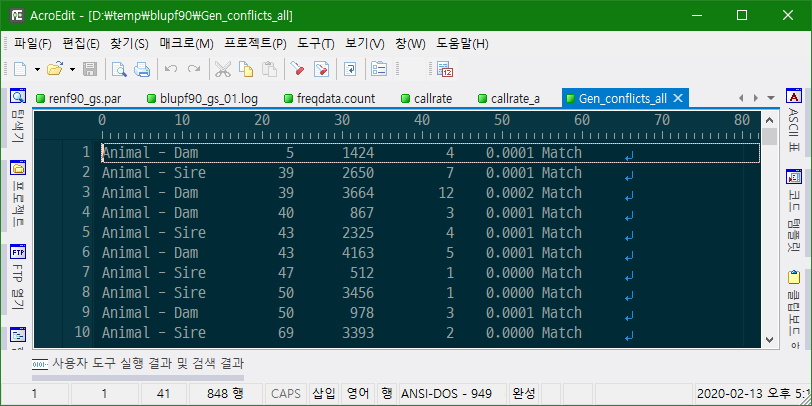
OPTION outparent_progeny
=> 친자감정 결과를 Gen_conflicts_all 파일에 남긴다.
옵션을 살펴보고 필요하면 추가한다.

blupf90 실행명령어와 실행화면은 다음과 같다.
|
blupf90 renf90_gs.par | tee blupf90_gs_01.log |

화면에 출력된 로그는 다음과 같다.
renf90_gs.par
BLUPF90 ver. 1.66
Parameter file: renf90_gs.par
Data file: renf90.dat
Number of Traits 1
Number of Effects 2
Position of Observations 1
Position of Weight (1) 0
Value of Missing Trait/Observation 0
=> 파라미터 파일, 자료 파일, 형질과 효과의 개수, 관측치 위치, missing value
EFFECTS
# type position (2) levels [positions for nested]
1 cross-classified 2 1
2 cross-classified 3 5384
=> 2열, 3열 효과와 레벨 개수
Residual (co)variance Matrix
0.62800
=> 잔차 분산
Random Effect(s) 2
Type of Random Effect: additive animal
Pedigree File: renadd02.ped
=> 개체 효과, 혈통 파일
trait effect (CO)VARIANCES
1 2 0.1438
=> 개체 효과의 분산
REMARKS
(1) Weight position 0 means no weights utilized
(2) Effect positions of 0 for some effects and traits means that such
effects are missing for specified traits
* convergence criterion (default=1e-12): 1.0000000E-12
* store solutions and s.e. *** se
* sparse package: YAMS
Options read from parameter file:
* SNP format: BLUPF90 standard (text)
* SNP file: 50k_for_gs.txt
* SNP Xref file: 50k_for_gs.txt_XrefID
* Map file: snp_map_for_gs.txt
* print call rate information for Locus and Individuals
* print parent_progeny information
* Use Animals with call rate > call rate (default call rate = 0.9): 0.90
* Save Clean SNP data to (SNP_file)_clean file (default .false.)
* Exclude Chromosomes (default .false.): 30 31 32
* Verify parent-progeny (default 3): 3
* use YAMS package for sparse computation (default=.false.)
*********************************************************
** OPTION chrinfo <file> is deprecated !! **
** **
** Use OPTION map_file <file> instead !! **
** **
** The <file> should has a header with the **
** following column names (no specific order): **
** SNP_ID identification of the SNP (alphanumeric) **
** CHR chromosome (numeric) **
** POS position (bp ) **
** Extra columns are possible **
*********************************************************
=> chrinfo 옵션은 곧 지원을 하지 않을 것이므로, map_file 옵션을 사용하라.
Data record length = 3
# equations = 5385
G
0.14380
read 3591 records in 0.5156250 s, 7183
nonzeroes
read 5384 additive pedigrees
*--------------------------------------------------------------*
* Genomic Library: Dist Version 1.268 *
* *
* Optimized OpenMP Version - 24 threads *
* *
* Modified relationship matrix (H) created for effect: 2 *
*--------------------------------------------------------------*
=> Genomic Library를 실행한다. pregsf90에서 수행한 것을 수행한다. pregsf90을 미리 하는 이유는 프로그램이 자동적으로 하는 것에 맡기기 보다는 에러를 살펴 보고 raw data를 수정해서 반복적으로 분석할 때 문제가 없게 하라는 의미이다.

아래 과정은 위 그림의 H 역행렬을 만드는 과정이다. A의 역행렬을 만들어야 한다. G = alpha * G + beat * A22를 만들어 G의 역행렬을 만든다. 여기서 alpha는 0.95, beta는 0.05인데 이 비율을 조정할 경우 최종적인 육종가 정확도에 영향을 미친다. 또 G의 역행렬과 A22의 역행렬을 만들어 H 역행렬을 만들 때 tau와 omega를 조종하면 육종가 정확도에 또한 영향을 미친다. 다음은 SNP 유전자형을 이용하여 결국에는 H 역행렬을 만드는 과정이다.
Read 5384 animals from pedigree file: "D:\temp\blupf90\renadd02.ped"
Number of Genotyped Animals: 1577
Creating A22
Extracting subset of: 2307 pedigrees from: 5384 elapsed time: 0.0000
Calculating A22 Matrix by Colleau OpenMP...elapsed time: .0134
Numbers of threads=1 24
Reading SNP file
Column position in file for the first marker: 17
Format to read SNP file: (16x,400000i1)
Number of SNPs: 51857
Format: integer genotypes (0 to 5) to double-precision array
Number of Genotyped animals: 1577
Reading SNP file elapsed time: 4.72
Statistics of alleles frequencies in the current population
N: 51857
Mean: 0.549
Min: 0.000
Max: 1.000
Var: 0.097
Reading MAP file: "snp_map_for_gs.txt" - 51857 SNPs out of 51857
Min and max # of chromosome: 1 29
Min and max # of SNP: 1 51857
Excluded 0 SNPs from 3 chromosomes: 30 31 32
Quality Control - SNPs with Call Rate < callrate ( 0.90) will removed: 0
Quality Control - SNPs with MAF < minfreq ( 0.05) will removed: 9293
Quality Control - Monomorphic SNPs will be removed: 1179
Quality Control - Removed Animals with Call rate < callrate ( 0.90): 0
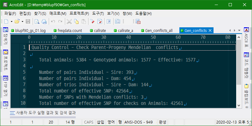
Quality Control - Check Parent-Progeny Mendelian conflicts
Total animals: 5384 - Genotyped animals: 1577 - Effective: 1577
Number of pairs Individual - Sire: 393
Number of pairs Individual - Dam: 454
Number of trios Individual - Sire - Dam: 144
No sex Chromosome information is available
Parent-progeny conflicts or HWE could eliminate SNPs in sex Chr
Provide map information and sex Chr to checks using autosomes
Checking SNPs for Mendelian conflicts
Total number of effective SNP: 42564
Total number of parent-progeny evaluations: 847
Number of SNPs with Mendelian conflicts: 3
Checking Animals for Mendelian conflicts
Total number of effective SNP for checks on Animals: 42561
Number of Parent-Progeny Mendelian Conflicts: 0
Number of effective SNPs (after QC): 42561
Number of effective Indiviuals (after QC): 1577
Statistics of alleles frequencies in the current population after
Quality Control (MAF, monomorphic, call rate, HWE, Mendelian conflicts)
N: 42561
Mean: 0.532
Min: 0.050
Max: 0.950
Var: 0.070
List of SNPs removed in: "50k_for_gs.txt_SNPs_removed"
Clean genotype file was created: "50k_for_gs.txt_clean"
Cross reference ID file was created: "50k_for_gs.txt_clean_XrefID"
Genotypes missings (%): 17.926
Genotypes missings after cleannig (%): 0.000
Calculating G Matrix
Dgemm MKL #threads= 1 24 Elapsed omp_get_time: 123.0466
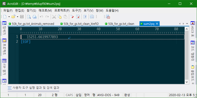
Scale by Sum(2pq). Average: 15251.6619977893
Detecting samples with similar genotypes
elapsed time= 0.0
Blend G as alpha*G + beta*A22: (alpha,beta) 0.950 0.050
Tuning: Scale G matrix according to A22 - Method: 2
Diagonal A: 1.002 Offdiagonal A: 0.003 All A: 0.004 Difference: 0.998
Diagonal G: 1.010 Offdiagonal G: -0.000 All G: 0.000 Difference: 1.010
Diff G Diag - G OffDiag: 1.010 (da-oa)/(dg-og): 0.988
Diff A OffDiag - G OffDiag: 0.004
Diff A all - G all: 0.004
New Alpha: 0.939 New Beta: 0.049
a + G*b; a: 0.004 b: 0.988
Method to select individuals: 1
Number of individual selected: 1577
Frequency - Diagonal of G
N: 1577
Mean: 1.002
Min: 0.739
Max: 1.384
Range: 0.032
Class: 20
#Class Class Count
1 0.7394 3
2 0.7717 1
3 0.8039 4
4 0.8362 2
5 0.8684 0
6 0.9006 0
7 0.9329 242
8 0.9651 724
9 0.9974 331
10 1.030 115
11 1.062 52
12 1.094 33
13 1.126 29
14 1.159 16
15 1.191 10
16 1.223 5
17 1.255 6
18 1.288 0
19 1.320 3
20 1.352 1
21 1.384 0
Check for diagonal of genomic relationship matrix
Check for diagonal of genomic relationship matrix, genotypes not removed: 0
------------------------------
Final Pedigree-Based Matrix
------------------------------
Statistic of Rel. Matrix A22
N Mean Min Max Var
Diagonal 1577 1.002 1.000 1.250 0.000
Off-diagonal 2485352 0.003 0.000 0.750 0.001
----------------------
Final Genomic Matrix
----------------------
Statistic of Genomic Matrix
N Mean Min Max Var
Diagonal 1577 1.002 0.739 1.384 0.003
Off-diagonal 2485352 0.003 -0.071 1.055 0.002
Correlation of Genomic Inbreeding and Pedigree Inbreeding
Correlation: 0.2199
All elements - Diagonal / Off-Diagonal
Estimating Regression Coefficients G = b0 11' + b1 A + e
Regression coefficients b0 b1 = 0.000 0.996
Correlation all elements G & A 0.723
Off-Diagonal
Using 62988 elements from A22 >= .02000
Estimating Regression Coefficients G = b0 11' + b1 A + e
Regression coefficients b0 b1 = 0.007 0.957
Correlation Off-Diagonal elements G & A 0.872
Creating A22-inverse
Inverse LAPACK MKL dpotrf/i #threads= 1 24 Elapsed omp_get_time: 0.5488
----------------------
Final A22 Inv Matrix
----------------------
Statistic of Inv. Rel. Matrix A22
N Mean Min Max Var
Diagonal 1577 1.575 1.000 14.240 0.812
Off-diagonal 2485352 -0.001 -1.167 1.500 0.001
Creating G-inverse
Inverse LAPACK MKL dpotrf/i #threads= 1 24 Elapsed omp_get_time: 1.1807
--------------------------
Final Genomic Inv Matrix
--------------------------
Statistic of Inv. Genomic Matrix
N Mean Min Max Var
Diagonal 1577 2.209 0.851 16.579 1.285
Off-diagonal 2485352 -0.001 -3.630 2.691 0.002
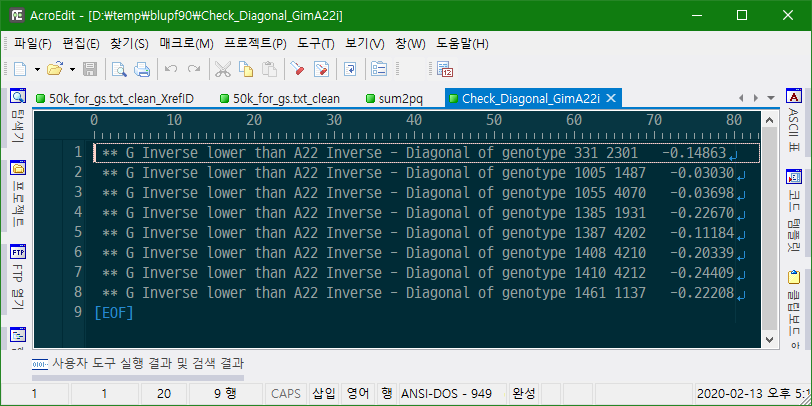
Check for diagonal of Inverse Genomic - Inverse of pedigree relationship matrix
Number of genotypes with G^ii < A22^ii: 8
Genotype number, renumber id and Gi-A22i print in file: "Check_Diagonal_GimA22i"
------------------------------
Final G Inv - A22 Inv Matrix
------------------------------
Statistic of Inv. Genomic- A22 Matrix
N Mean Min Max Var
Diagonal 1577 0.634 -0.244 4.172 0.139
Off-diagonal 2485352 -0.001 -3.630 1.732 0.001
*--------------------------------------------------*
* Setup Genomic Done !!!, elapsed time: 147.109 *
*--------------------------------------------------*
hash matrix increased from 131072 to 262144 % filled: 0.8000
hash matrix increased from 262144 to 524288 % filled: 0.8000
hash matrix increased from 524288 to 1048576 % filled: 0.8000
hash matrix increased from 1048576 to 2097152 % filled: 0.8000
finished peds in 176.5781 s, 1258483 nonzeroes
solutions and s.e. stored in file: "solutions"
blupf90을 실행하여 다음과 같은 파일들이 생긴다.

freqdata.count

callrate

callrate_a

Gen_conflicts_all
Gen_conflicts
freqdata.count.after.clean

snp_map_for_gs.txt_clean

50k_for_gs.txt_SNPs_removed

50k_for_gs.txt_Animals_removed
=> 이번 분석에서는 빈 파일
50k_for_gs.txt_clean_XrefID
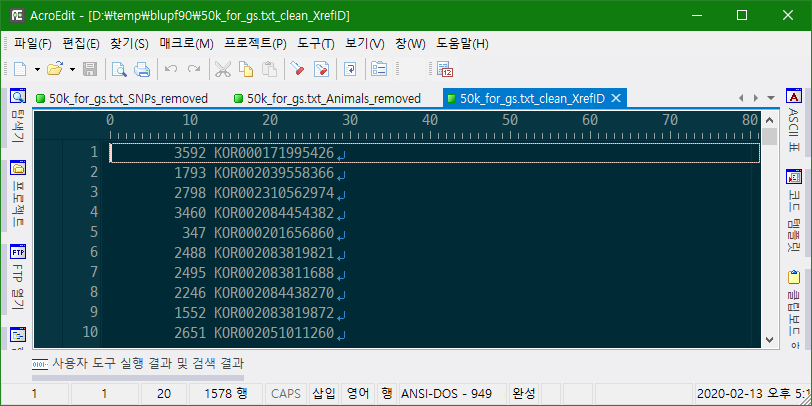
50k_for_gs.txt_clean

sum2pq
Check_Diagonal_GimA22i
solutions
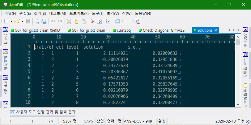
육종가의 표준 오차를 이용하여 정확도를 계산한다. SNP 유전체 자료를 넣었을 때, 안 넣었을 때 정확도를 비교하여 SNP 유전체 자료의 효용성에 대해서 비교한다. 검정 자료는 가지고 있지 않고 유전체 자료만 가진 개체를 포함하여 본 프로세스를 진행할 경우 즉 가축이 태어난 직후 관련 검정 자료는 없고, 오로지 유전체 자료만 가질 때 본 프로세스를 진행하여 해당 개체의 육종가 정확도를 보고 유전체 선발의 적용을 생각할 수 있다.
'Animal Breeding > Genomic Selection' 카테고리의 다른 글
| PostGSF90을 이용한 GWAS (0) | 2020.03.05 |
|---|---|
| SNP Marker Effect 추정 (0) | 2020.03.02 |
| SNP 유전체 자료를 이용한 아비 어미 찾기 (0) | 2020.02.12 |
| QCF90이용한 quality control (0) | 2020.02.05 |
| PREGSF90을 이용한 Quality Control (0) | 2020.02.04 |