앞에서는 각 형질의 모형이 같다고 가정하였다. 즉 각 형질에 동일한 고정 효과와 임의 효과(effect)가 들어간다는 뜻이다. 각 형질의 모형이 다를 때, 즉 모형에 포함된 효과(effect)가 다른 경우를 다룬다. 예를 들어 hys1은 첫번째 형질에만 해당되고, hys2는 두번째 형질에만 해당되는 경우이다. 비록 모형이 다르더라도 모형이 같다고 가정해야 traits in animal(effect) 방식으로 프로그램을 할 수 있다.
예를 들어 자료가 다음과 같다고 가정하자.
4 1 1 201 280
5 1 2 150 200
6 2 1 160 190
7 1 1 180 250
8 2 2 285 300
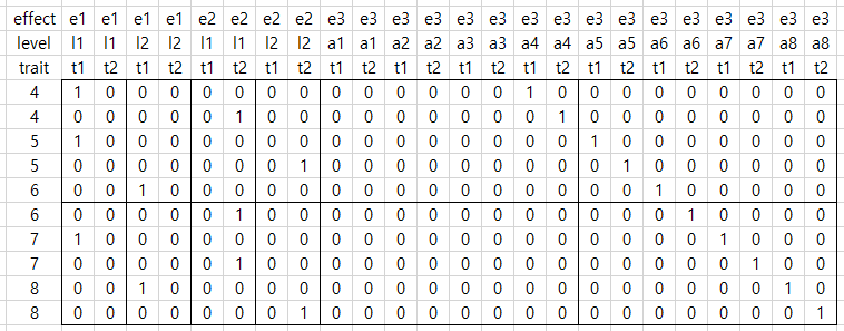
첫째 컬럼은 animal이다. 둘째 컬럼은 hys1인데 첫째 형질의 모형에만 들어간다. 셋째 컬럼은 hys2인데 둘째 형질의 모형에만 들어간다. 넷째는 fat1으로 1산 유지량 형질, 다섯째는 fat2로 2산 유지량이다. 비록 hys1이 첫째 형질에만 hys2가 둘째 형질에만 있지만, 두 고정효과 모두 양 쪽 형질의 모형에 있다고 가정한다. 그래서 same model이라고 하면 다음과 같이 design matrix가 만들어질 것이다.

그러나 사실 hys1은 형질 2에 없고, hys2는 형질 1에 없으므로 다음과 같이 만들어진다.

위는 효과 내에, 형질 내에, 레벨이 나오는데 이것은 형질 -> 레벨 -> 형질의 순으로 바꾸어 생각한다.
위의 design matrix에서 4번 개체가 LHS에 기여하는 바는 다음과 같다. R의 inverse를 곱하여 얻은 값이다.

총 9개의 네 모칸이 나오는데 그것은 hys1, hys2, animal 각각 교차하여 차지하는 칸이다. 그런데 hys1은 첫째 형질의 모형에만 있으므로 R의 inverse 앞 뒤에 [ [ 1, 0], [0, 0] ]을 곱하여 준다. 구체적으로 다음과 같다.

같은 방식으로 RHS를 채우고, 나머지 개체들도 같은 방식으로 LHS와 RHS를 채운다.
# multiple trait animal model, unequal design matrices(different model) - Date : 2020-07-29
# Linear Models for the Prediction of Animal Breeding Values, 3rd Edtion
# Raphael Mrode
# Example 5.3 p80
위의 예를 가지고 R로 육종가를 구하고, 정확도를 구하고, 육종가를 분할하고, DYD를 계산한 것을 설명한다.
자료는 다음과 같다.
4 1 1 201 280
5 1 2 150 200
6 2 1 160 190
7 1 1 180 250
8 2 2 285 300
mt03_data.txt로 저장한다. 컬럼 설명은 위에서 하였다.
혈통은 다음과 같다.
1 0 0
2 0 0
3 0 0
4 1 2
5 3 2
6 1 5
7 3 4
8 1 7
mt3_pedi.txt로 저장한다.
R 프로그램은 다음과 같다.
# multiple trait animal model, unequal design matrices(different model) - Date : 2020-07-29

# Linear Models for the Prediction of Animal Breeding Values, 3rd Edtion

# Raphael Mrode

# Example 5.3 p80

# MASS packages
if (!("MASS" %in% installed.packages())) {
    install.packages("MASS", dependencies = TRUE)
}
library(MASS)

# functions

# find the position in mixed model equation(lhs and rhs)
pos_mme <- function(trts, lvls, vals) {
    pos = rep(0, length(vals))

    for (i in 1:length(vals)) {
        if (i == 1) {
            pos[i] = trts * (vals[i] - 1) + 1
        } else {
            pos[i] = trts * sum(lvls[1:i - 1]) + trts * (vals[i] - 1) + 1
        }
    }

    return(pos)
}

# make design matrix
desgn <- function(v) {
    if (is.numeric(v)) {
        va = v
        mrow = length(va)
        mcol = max(va)
    }
    if (is.character(v)) {
        vf = factor(v)
        # 각 수준의 인덱스 값을 저장
        va = as.numeric(vf)
        mrow = length(va)
        mcol = length(levels(vf))
    }

    # 0으로 채워진 X 준비
    X = matrix(data = c(0), nrow = mrow, ncol = mcol)

    for (i in 1:mrow) {
        ic = va[i]
        X[i, ic] = 1
    }
    return(X)
}

# function to make inverse of numerator relationship matrix
ainv = function(pedi) {
    n = nrow(pedi)
    Ainv = matrix(c(0), nrow = n, ncol = n)

    for (i in 1:n) {
        animal = pedi[i, 1]
        sire = pedi[i, 2]
        dam = pedi[i, 3]

        if (sire == 0 & dam == 0) {
            # both parents unknown
            alpha = 1
            Ainv[animal, animal] = alpha + Ainv[animal, animal]
        } else if (sire != 0 & dam == 0) {
            # sire known
            alpha = 4/3
            Ainv[animal, animal] = alpha + Ainv[animal, animal]
            Ainv[animal, sire] = -alpha/2 + Ainv[animal, sire]
            Ainv[sire, animal] = -alpha/2 + Ainv[sire, animal]
            Ainv[sire, sire] = alpha/4 + Ainv[sire, sire]
        } else if (sire == 0 & dam != 0) {
            # dam known
            alpha = 4/3
            Ainv[animal, animal] = alpha + Ainv[animal, animal]
            Ainv[animal, dam] = -alpha/2 + Ainv[animal, dam]
            Ainv[dam, animal] = -alpha/2 + Ainv[dam, animal]
            Ainv[dam, dam] = alpha/4 + Ainv[dam, dam]
        } else {
            # both parents known
            alpha = 2
            Ainv[animal, animal] = alpha + Ainv[animal, animal]
            Ainv[animal, sire] = -alpha/2 + Ainv[animal, sire]
            Ainv[sire, animal] = -alpha/2 + Ainv[sire, animal]
            Ainv[animal, dam] = -alpha/2 + Ainv[animal, dam]
            Ainv[dam, animal] = -alpha/2 + Ainv[dam, animal]
            Ainv[sire, sire] = alpha/4 + Ainv[sire, sire]
            Ainv[sire, dam] = alpha/4 + Ainv[sire, dam]
            Ainv[dam, sire] = alpha/4 + Ainv[dam, sire]
            Ainv[dam, dam] = alpha/4 + Ainv[dam, dam]
        }
    }
    return(Ainv)
}

# set working directory
#setwd(choose.dir())
setwd("D:/temp/06_multiple_traits_03_R")

# print working directory
getwd()

# no_of_trts
no_trts = 2

# list all possible combination of data
dtcombi0 = expand.grid(rep(list(0:1), no_trts))
dtcombi = dtcombi0[2:nrow(dtcombi0), ]
rownames(dtcombi) = NULL

# print
dtcombi

# prdigree and data

# read pedigree : animal sire dam
pedi = read.table("mt03_pedi.txt", header = FALSE, sep = "", col.names = c("animal", "sire", "dam"),
    stringsAsFactors = FALSE)
pedi = pedi[order(pedi$animal), ]

# print
pedi

# read data : animal, dam, sex, weaning_weight
data = read.table("mt03_data.txt", header = FALSE, sep = "", col.names = c("animal", "hys1", "hys2", "fat1", "fat2"),
    stringsAsFactors = FALSE)

# print
data

# number of data
no_data = nrow(data)

# print
no_data

# how many traits does animal have?
data2 = data.frame(data, dtsts = c(0))
data2$dtsts = ifelse(data2$fat1 != 0, data2$dtsts + 1, data2$dtsts)
data2$dtsts = ifelse(data2$fat2 != 0, data2$dtsts + 2, data2$dtsts)

# print
data2

# levels of animal, hys1, hys2
lvls_hys1 = max(data2$hys1)
lvls_hys2 = max(data2$hys2)
lvls_ani = max(data2$animal)

# print
lvls_hys1
lvls_hys2
lvls_ani

# effect data status. 1st effect(hys1) is for trait 1, 2nd effect(hys2) is for trait 2, 3rd effect is for trait 1 and 2.
effdtsts = array(rep(0, no_trts * no_trts * (2^no_trts - 1)), dim = c(no_trts, no_trts, (2^no_trts - 1)))
effdtsts[,,1] = diag(c(1,0))
effdtsts[,,2] = diag(c(0,1))
effdtsts[,,3] = diag(c(1,1))

# print
effdtsts

# variance component additive genetic
G = matrix(c(35, 28, 28, 30), 2, 2)
# residual
R = matrix(c(65, 27, 27, 70), 2, 2)

# print
G
R

# inverse of G
Gi = ginv(G)

# print
Gi

# inverse of R
Ri = array(rep(0, no_trts * no_trts * (2^no_trts - 1)), dim = c(no_trts, no_trts, (2^no_trts - 1)))

for (i in 1:(2^no_trts - 1)) {
    R0 = R
    R0[which(dtcombi[i, ] == 0), ] = 0
    R0[, which(dtcombi[i, ] == 0)] = 0
    Ri[, , i] = ginv(R0)
}

# print
Ri

# empty lhs
lhs = matrix(rep(0, (no_trts * (lvls_hys1 + lvls_hys2 + lvls_ani))^2), nrow = no_trts * (lvls_hys1 + lvls_hys2 + lvls_ani))

# print
dim(lhs)
lhs

# empty rhs
rhs = matrix(rep(0, (no_trts * (lvls_hys1 + lvls_hys2 + lvls_ani))), nrow = no_trts * (lvls_hys1 + lvls_hys2 + lvls_ani))

# print
dim(rhs)
rhs

# fill the MME
for (i in 1:no_data) {
#i = 1
    pos = pos_mme(no_trts, c(lvls_hys1, lvls_hys2, lvls_ani), c(data2$hys1[i], data2$hys2[i], data2$animal[i]))

    for (j in 1:length(pos)) {
        rfirst = pos[j]
        rlast = (pos[j] + no_trts - 1)

        for (k in 1:length(pos)) {
            cfirst = pos[k]
            clast = (pos[k] + no_trts - 1)

            lhs[rfirst : rlast, cfirst : clast] = lhs[rfirst : rlast, cfirst : clast] + effdtsts[,,j] %*% Ri[, , data2$dtsts[i]] %*% effdtsts[,,k]
        }
        rhs[rfirst : rlast] = rhs[rfirst : rlast] + effdtsts[,,j] %*% Ri[, , data2$dtsts[i]] %*% as.numeric(data2[i, 4:5])
    }
}

# print lhs and rhs
lhs
rhs

# inverse matrix of NRM
ai = ainv(pedi)

# print
ai

# add ai to lhs
afirst = no_trts * lvls_hys1 * lvls_hys2 + 1
alast = no_trts * (lvls_hys1 * lvls_hys2 + lvls_ani)
afirst
alast
lhs[afirst : alast, afirst : alast] = lhs[afirst : alast, afirst : alast] + ai %x% Gi


# print
#lhs[c(2,4,5,7),] = 0
#lhs[,c(2,4,5,7)] = 0
#rhs[c(2,4,5,7),] = 0

lhs
rhs

# generalised inverse of lhs
gi_lhs = ginv(lhs)

# print
gi_lhs

# solution
sol = gi_lhs %*% rhs

# print
sol

# levels of fixed effect 1 in traits 1
lvls_t1_f1 = rep(0, lvls_hys1)
for ( i in 1 : lvls_hys1){
    if (i == 1){
        lvls_t1_f1[i] = 1
    } else {
        lvls_t1_f1[i] = 1 + (i - 1) * no_trts
    }
}

# print
lvls_t1_f1

# levels of fixed effect 1 in traits 2
lvls_t2_f1 = lvls_t1_f1 + 1

# print
lvls_t2_f1

# levels of fixed effect 2 in traits 1
lvls_t1_f2 = rep(0, lvls_hys2)
for ( i in 1 : lvls_hys2){
    if (i == 1){
        lvls_t1_f2[i] = 1
    } else {
        lvls_t1_f2[i] = 1 + (i - 1) * no_trts
    }
}

# print
lvls_t1_f2 = lvls_t1_f2 + no_trts * lvls_hys1
lvls_t1_f2

# levels of fixed effect 2 in traits 2
lvls_t2_f2 = lvls_t1_f2 + 1

# print
lvls_t2_f2

# levels of animal effect in traits 1
lvls_t1_ani = rep(0, lvls_ani)
for ( i in 1 : lvls_ani){
    if (i == 1){
        lvls_t1_ani[i] = 1
    } else {
        lvls_t1_ani[i] = 1 + (i - 1) * no_trts
    }
}
lvls_t1_ani = lvls_t1_ani + no_trts * (lvls_hys1 + lvls_hys2)

# print
lvls_t1_ani

# levels of fixed effect in traits 1
lvls_t2_ani = lvls_t1_ani + 1

# print
lvls_t2_ani

# solutions for fixed effects 1
sol_t1_f1 = as.matrix(sol[lvls_t1_f1])
sol_t2_f1 = as.matrix(sol[lvls_t2_f1])
sol_f1 = cbind(sol_t1_f1, sol_t2_f1)

# print
sol_f1

# solutions for fixed effects 2
sol_t1_f2 = as.matrix(sol[lvls_t1_f2])
sol_t2_f2 = as.matrix(sol[lvls_t2_f2])
sol_f2 = cbind(sol_t1_f2, sol_t2_f2)

# print
sol_f2

# breedinv value
sol_t1_bv = sol[lvls_t1_ani]
sol_t2_bv = sol[lvls_t2_ani]
sol_bv = cbind(sol_t1_bv, sol_t2_bv)

# print
sol_bv

# reliability(r2), accuracy(r), standard error of prediction(SEP)

# diagonal elements of the generalized inverse of LHS for animal equation
d_ani_t1 = diag(gi_lhs[lvls_t1_ani, lvls_t1_ani])
d_ani_t2 = diag(gi_lhs[lvls_t2_ani, lvls_t2_ani])
d_ani = cbind(d_ani_t1, d_ani_t2)

# print
d_ani

# reliability
rel = matrix(rep(0, lvls_ani * no_trts), ncol = no_trts)

for (i in 1 : lvls_ani) {
    rel[i, ] = 1 - d_ani[i, ]/diag(G)
}

# print
rel

# accuracy
acc = sqrt(rel)

# print
acc

# standard error of prediction(SEP)
sep = sqrt(d_ani)

# 확인
sep

# partitioning of breeding values

# yield deviation
yd1 = matrix(rep(0, lvls_ani * no_trts), ncol = no_trts)

# numerator of n2
a2 = array(rep(0, no_trts * no_trts * lvls_ani), dim = c(no_trts, no_trts, lvls_ani))

# looping data
for (i in 1:no_data) {
    yd1[data[i, 1], ] = as.matrix(data2[i, c(4, 5)] - sol_f1[data2[i, 2], ] - sol_f2[data2[i, 3], ])

    a2[, , data[i, 1]] = Ri[, , data2$dtsts[i]]
}

# print
yd1
a2

# Parents average, progeny contribution

# parents avearge
pa1 = matrix(rep(0, lvls_ani * no_trts), ncol = no_trts)

# progeny contribution numerator
pc0 = matrix(rep(0, lvls_ani * no_trts), ncol = no_trts)

# numerator of n3, denominator of progeny contribution
a3 = array(rep(0, no_trts * no_trts * lvls_ani), dim = c(no_trts, no_trts, lvls_ani))

# numerator of n1
a1 = array(rep(0, no_trts * no_trts * lvls_ani), dim = c(no_trts, no_trts, lvls_ani))


# looping pedi
for (i in 1 : lvls_ani) {

    sire = pedi[i, 2]
    dam = pedi[i, 3]

    if (sire == 0 & dam == 0) {
        # both parents unknown PA
        a1[, , i] = 1 * Gi

    } else if (sire != 0 & dam == 0) {
        # 개체의 부만 알고 있을 경우

        # PA
        a1[, , i] = 4/3 * Gi
        pa1[i, ] = sol_bv[sire, ]/2

        # PC for sire
        a3[, , sire] = a3[, , sire] + 0.5 * Gi * (2/3)
        pc0[sire, ] = pc0[sire, ] + (0.5 * Gi * (2/3)) %*% (2 * sol_bv[i, ])

    } else if (sire == 0 & dam != 0) {
        # dam known

        # PA
        a1[, , i] = 4/3 * Gi
        pa1[i, ] = sol_bv[dam, ]/2

        # PC for dam
        a3[, , dam] = a3[, , dam] + 0.5 * Gi * (2/3)
        pc0[dam, ] = pc0[dam, ] + (0.5 * Gi * (2/3)) %*% (2 * sol_bv[i])

    } else {
        # both parents known

        # PA
        a1[, , i] = 2 * Gi
        pa1[i, ] = (sol_bv[sire, ] + sol_bv[dam, ])/2

        # PC for sire
        a3[, , sire] = a3[, , sire] + 0.5 * Gi
        pc0[sire, ] = pc0[sire, ] + (0.5 * Gi) %*% (2 * sol_bv[i, ] - sol_bv[dam, ])

        # PC for dam
        a3[, , dam] = a3[, , dam] + 0.5 * Gi
        pc0[dam, ] = pc0[dam, ] + (0.5 * Gi) %*% (2 * sol_bv[i, ] - sol_bv[sire, ])

    }
}

# print
a1
pa1
a3
pc0

# denominator of n1, n2, n3, diagonal of animals in LHS
n_de = a1 + a2 + a3

# print
n_de

# parents average fraction of breeding values
pa = matrix(rep(0, lvls_ani * no_trts), ncol = no_trts)
for (i in 1 : lvls_ani) {
    pa[i, ] = ginv(n_de[, , i]) %*% a1[, , i] %*% pa1[i, ]
}

# print
pa

# yield deviation fraction of breeding values
yd = matrix(rep(0, lvls_ani * no_trts), ncol = no_trts)
for (i in 1 : lvls_ani) {
    yd[i, ] = ginv(n_de[, , i]) %*% a2[, , i] %*% yd1[i, ]
}

# print
yd

# progeny contribution
pc1 = matrix(rep(0, lvls_ani * no_trts), ncol = no_trts)
for (i in 1 : lvls_ani) {
    pc1[i, ] = ginv(a3[, , i]) %*% pc0[i, ]
}
pc1[is.nan(pc1) == TRUE] = 0
pc1

# progeny contribution fraction of breeding values
pc = matrix(rep(0, lvls_ani * no_trts), ncol = no_trts)
for (i in 1 : lvls_ani) {
    pc[i, ] = ginv(n_de[, , i]) %*% a3[, , i] %*% pc1[i, ]
}

# print
pc

# Progeny(Daughter) Yield Deviation(PYD, DYD)

# n2 of progeny
n2prog = array(rep(0, no_trts * no_trts * lvls_ani), dim = c(no_trts, no_trts, lvls_ani))
for (i in 1 : lvls_ani) {
    n2prog[, , i] = ginv((a1 + a2)[, , i]) %*% a2[, , i]
}

# print
n2prog

# numerator of dyd : summation of u of progeny * n2 of progeny * (2 * YD - bv of mate)
dyd_n = matrix(rep(0, lvls_ani * no_trts), ncol = no_trts)
# denominator of dyd : summation of u of progeny * n2 of progeny
dyd_d = array(rep(0, no_trts * no_trts * lvls_ani), dim = c(no_trts, no_trts, lvls_ani))

# looping pedi
for (i in 1 : lvls_ani) {
    # i = 5
    sire = pedi[i, 2]
    dam = pedi[i, 3]

    if (sire == 0 & dam == 0) {
        # both parents unknown

    } else if (sire != 0 & dam == 0) {
        # 개체의 부만 알고 있을 경우

        # dyd_n
        dyd_n[sire, ] = dyd_n[sire, ] + (n2prog[, , i] * 2/3) %*% (2 * yd1[i, ])
        # dyd_d
        dyd_d[, , sire] = dyd_d[, , sire] + n2prog[, , i] * 2/3

    } else if (sire == 0 & dam != 0) {
        # dam known

        # dyd_n
        dyd_n[dam, ] = dyd_n[dam, ] + (n2prog[, , i] * 2/3) %*% (2 * yd1[i, ])
        # dyd_d
        dyd_d[, , dam] = dyd_d[, , dam] + n2prog[, , i] * 2/3

    } else {
        # both parents known

        # dyd_n
        dyd_n[sire, ] = dyd_n[sire, ] + n2prog[, , i] %*% (2 * yd1[i, ] - sol_bv[dam, ])
        dyd_n[dam, ] = dyd_n[dam, ] + n2prog[, , i] %*% (2 * yd1[i, ] - sol_bv[sire, ])

        # dyd_d
        dyd_d[, , sire] = dyd_d[, , sire] + n2prog[, , i]
        dyd_d[, , dam] = dyd_d[, , dam] + n2prog[, , i]

    }
}

# print
dyd_n
dyd_d

# dyd
dyd = matrix(rep(0, lvls_ani * no_trts), ncol = no_trts)

# looping pedi
for (i in 1 : lvls_ani) {
    dyd[i, ] = ginv(dyd_d[, , i]) %*% dyd_n[i, ]
}
dyd[is.nan(dyd) == TRUE] = 0

# print
dyd

# breeding values and fractions
mt3_result = data.frame(animal = pedi[, 1], animal_bv = sol_bv, rel = rel, acc = acc, sep = sep, pa = pa,
    yd = yd, pc = pc, sum_of_fr = pa + yd + pc, dyd = dyd)

# print
mt3_result

# 파일로 출력, 분리자는 ',', 따옴표 없고
output_filename = gsub("[ -]", "", paste("mt3_result_", Sys.Date(), ".csv"))
write.table(mt3_result, output_filename, sep = ",", row.names = FALSE, quote = FALSE)
실행결과는 다음과 같다.
> # multiple trait animal model, unequal design matrices(different model) - Date : 2020-07-29
>
> # Linear Models for the Prediction of Animal Breeding Values, 3rd Edtion
>
> # Raphael Mrode
>
> # Example 5.3 p80
>
> # MASS packages
> if (!("MASS" %in% installed.packages())) {
+ install.packages("MASS", dependencies = TRUE)
+ }
> library(MASS)
>
> # functions
>
> # find the position in mixed model equation(lhs and rhs)
> pos_mme <- function(trts, lvls, vals) {
+ pos = rep(0, length(vals))
+
+ for (i in 1:length(vals)) {
+ if (i == 1) {
+ pos[i] = trts * (vals[i] - 1) + 1
+ } else {
+ pos[i] = trts * sum(lvls[1:i - 1]) + trts * (vals[i] - 1) + 1
+ }
+ }
+
+ return(pos)
+ }
>
> # make design matrix
> desgn <- function(v) {
+ if (is.numeric(v)) {
+ va = v
+ mrow = length(va)
+ mcol = max(va)
+ }
+ if (is.character(v)) {
+ vf = factor(v)
+ # 각 수준의 인덱스 값을 저장
+ va = as.numeric(vf)
+ mrow = length(va)
+ mcol = length(levels(vf))
+ }
+
+ # 0으로 채워진 X 준비
+ X = matrix(data = c(0), nrow = mrow, ncol = mcol)
+
+ for (i in 1:mrow) {
+ ic = va[i]
+ X[i, ic] = 1
+ }
+ return(X)
+ }
>
> # function to make inverse of numerator relationship matrix
> ainv = function(pedi) {
+ n = nrow(pedi)
+ Ainv = matrix(c(0), nrow = n, ncol = n)
+
+ for (i in 1:n) {
+ animal = pedi[i, 1]
+ sire = pedi[i, 2]
+ dam = pedi[i, 3]
+
+ if (sire == 0 & dam == 0) {
+ # both parents unknown
+ alpha = 1
+ Ainv[animal, animal] = alpha + Ainv[animal, animal]
+ } else if (sire != 0 & dam == 0) {
+ # sire known
+ alpha = 4/3
+ Ainv[animal, animal] = alpha + Ainv[animal, animal]
+ Ainv[animal, sire] = -alpha/2 + Ainv[animal, sire]
+ Ainv[sire, animal] = -alpha/2 + Ainv[sire, animal]
+ Ainv[sire, sire] = alpha/4 + Ainv[sire, sire]
+ } else if (sire == 0 & dam != 0) {
+ # dam known
+ alpha = 4/3
+ Ainv[animal, animal] = alpha + Ainv[animal, animal]
+ Ainv[animal, dam] = -alpha/2 + Ainv[animal, dam]
+ Ainv[dam, animal] = -alpha/2 + Ainv[dam, animal]
+ Ainv[dam, dam] = alpha/4 + Ainv[dam, dam]
+ } else {
+ # both parents known
+ alpha = 2
+ Ainv[animal, animal] = alpha + Ainv[animal, animal]
+ Ainv[animal, sire] = -alpha/2 + Ainv[animal, sire]
+ Ainv[sire, animal] = -alpha/2 + Ainv[sire, animal]
+ Ainv[animal, dam] = -alpha/2 + Ainv[animal, dam]
+ Ainv[dam, animal] = -alpha/2 + Ainv[dam, animal]
+ Ainv[sire, sire] = alpha/4 + Ainv[sire, sire]
+ Ainv[sire, dam] = alpha/4 + Ainv[sire, dam]
+ Ainv[dam, sire] = alpha/4 + Ainv[dam, sire]
+ Ainv[dam, dam] = alpha/4 + Ainv[dam, dam]
+ }
+ }
+ return(Ainv)
+ }
>
> # set working directory
> #setwd(choose.dir())
> setwd("D:/temp/06_multiple_traits_03_R")
>
> # print working directory
> getwd()
[1] "D:/temp/06_multiple_traits_03_R"
>
> # no_of_trts
> no_trts = 2
>
> # list all possible combination of data
> dtcombi0 = expand.grid(rep(list(0:1), no_trts))
> dtcombi = dtcombi0[2:nrow(dtcombi0), ]
> rownames(dtcombi) = NULL
>
> # print
> dtcombi
Var1 Var2
1 1 0
2 0 1
3 1 1
>
> # prdigree and data
>
> # read pedigree : animal sire dam
> pedi = read.table("mt03_pedi.txt", header = FALSE, sep = "", col.names = c("animal", "sire", "dam"),
+ stringsAsFactors = FALSE)
> pedi = pedi[order(pedi$animal), ]
>
> # print
> pedi
animal sire dam
1 1 0 0
2 2 0 0
3 3 0 0
4 4 1 2
5 5 3 2
6 6 1 5
7 7 3 4
8 8 1 7
>
> # read data : animal, dam, sex, weaning_weight
> data = read.table("mt03_data.txt", header = FALSE, sep = "", col.names = c("animal", "hys1", "hys2", "fat1", "fat2"),
+ stringsAsFactors = FALSE)
>
> # print
> data
animal hys1 hys2 fat1 fat2
1 4 1 1 201 280
2 5 1 2 150 200
3 6 2 1 160 190
4 7 1 1 180 250
5 8 2 2 285 300
>
> # number of data
> no_data = nrow(data)
>
> # print
> no_data
[1] 5
>
> # how many traits does animal have?
> data2 = data.frame(data, dtsts = c(0))
> data2$dtsts = ifelse(data2$fat1 != 0, data2$dtsts + 1, data2$dtsts)
> data2$dtsts = ifelse(data2$fat2 != 0, data2$dtsts + 2, data2$dtsts)
>
> # print
> data2
animal hys1 hys2 fat1 fat2 dtsts
1 4 1 1 201 280 3
2 5 1 2 150 200 3
3 6 2 1 160 190 3
4 7 1 1 180 250 3
5 8 2 2 285 300 3
>
> # levels of animal, hys1, hys2
> lvls_hys1 = max(data2$hys1)
> lvls_hys2 = max(data2$hys2)
> lvls_ani = max(data2$animal)
>
> # print
> lvls_hys1
[1] 2
> lvls_hys2
[1] 2
> lvls_ani
[1] 8
>
> # effect data status. 1st effect(hys1) is for trait 1, 2nd effect(hys2) is for trait 2, 3rd effect is for trait 1 and 2.
> effdtsts = array(rep(0, no_trts * no_trts * (2^no_trts - 1)), dim = c(no_trts, no_trts, (2^no_trts - 1)))
> effdtsts[,,1] = diag(c(1,0))
> effdtsts[,,2] = diag(c(0,1))
> effdtsts[,,3] = diag(c(1,1))
>
> # print
> effdtsts
, , 1
[,1] [,2]
[1,] 1 0
[2,] 0 0
, , 2
[,1] [,2]
[1,] 0 0
[2,] 0 1
, , 3
[,1] [,2]
[1,] 1 0
[2,] 0 1
>
> # variance component additive genetic
> G = matrix(c(35, 28, 28, 30), 2, 2)
> # residual
> R = matrix(c(65, 27, 27, 70), 2, 2)
>
> # print
> G
[,1] [,2]
[1,] 35 28
[2,] 28 30
> R
[,1] [,2]
[1,] 65 27
[2,] 27 70
>
> # inverse of G
> Gi = ginv(G)
>
> # print
> Gi
[,1] [,2]
[1,] 0.1127820 -0.1052632
[2,] -0.1052632 0.1315789
>
> # inverse of R
> Ri = array(rep(0, no_trts * no_trts * (2^no_trts - 1)), dim = c(no_trts, no_trts, (2^no_trts - 1)))
>
> for (i in 1:(2^no_trts - 1)) {
+ R0 = R
+ R0[which(dtcombi[i, ] == 0), ] = 0
+ R0[, which(dtcombi[i, ] == 0)] = 0
+ Ri[, , i] = ginv(R0)
+ }
>
> # print
> Ri
, , 1
[,1] [,2]
[1,] 0.01538462 0
[2,] 0.00000000 0
, , 2
[,1] [,2]
[1,] 0 0.00000000
[2,] 0 0.01428571
, , 3
[,1] [,2]
[1,] 0.018319812 -0.007066213
[2,] -0.007066213 0.017011254
>
> # empty lhs
> lhs = matrix(rep(0, (no_trts * (lvls_hys1 + lvls_hys2 + lvls_ani))^2), nrow = no_trts * (lvls_hys1 + lvls_hys2 + lvls_ani))
>
> # print
> dim(lhs)
[1] 24 24
> lhs
[,1] [,2] [,3] [,4] [,5] [,6] [,7] [,8] [,9] [,10] [,11] [,12] [,13] [,14] [,15] [,16] [,17] [,18] [,19] [,20] [,21]
[1,] 0 0 0 0 0 0 0 0 0 0 0 0 0 0 0 0 0 0 0 0 0
[2,] 0 0 0 0 0 0 0 0 0 0 0 0 0 0 0 0 0 0 0 0 0
[3,] 0 0 0 0 0 0 0 0 0 0 0 0 0 0 0 0 0 0 0 0 0
[4,] 0 0 0 0 0 0 0 0 0 0 0 0 0 0 0 0 0 0 0 0 0
[5,] 0 0 0 0 0 0 0 0 0 0 0 0 0 0 0 0 0 0 0 0 0
[6,] 0 0 0 0 0 0 0 0 0 0 0 0 0 0 0 0 0 0 0 0 0
[7,] 0 0 0 0 0 0 0 0 0 0 0 0 0 0 0 0 0 0 0 0 0
[8,] 0 0 0 0 0 0 0 0 0 0 0 0 0 0 0 0 0 0 0 0 0
[9,] 0 0 0 0 0 0 0 0 0 0 0 0 0 0 0 0 0 0 0 0 0
[10,] 0 0 0 0 0 0 0 0 0 0 0 0 0 0 0 0 0 0 0 0 0
[11,] 0 0 0 0 0 0 0 0 0 0 0 0 0 0 0 0 0 0 0 0 0
[12,] 0 0 0 0 0 0 0 0 0 0 0 0 0 0 0 0 0 0 0 0 0
[13,] 0 0 0 0 0 0 0 0 0 0 0 0 0 0 0 0 0 0 0 0 0
[14,] 0 0 0 0 0 0 0 0 0 0 0 0 0 0 0 0 0 0 0 0 0
[15,] 0 0 0 0 0 0 0 0 0 0 0 0 0 0 0 0 0 0 0 0 0
[16,] 0 0 0 0 0 0 0 0 0 0 0 0 0 0 0 0 0 0 0 0 0
[17,] 0 0 0 0 0 0 0 0 0 0 0 0 0 0 0 0 0 0 0 0 0
[18,] 0 0 0 0 0 0 0 0 0 0 0 0 0 0 0 0 0 0 0 0 0
[19,] 0 0 0 0 0 0 0 0 0 0 0 0 0 0 0 0 0 0 0 0 0
[20,] 0 0 0 0 0 0 0 0 0 0 0 0 0 0 0 0 0 0 0 0 0
[21,] 0 0 0 0 0 0 0 0 0 0 0 0 0 0 0 0 0 0 0 0 0
[22,] 0 0 0 0 0 0 0 0 0 0 0 0 0 0 0 0 0 0 0 0 0
[23,] 0 0 0 0 0 0 0 0 0 0 0 0 0 0 0 0 0 0 0 0 0
[24,] 0 0 0 0 0 0 0 0 0 0 0 0 0 0 0 0 0 0 0 0 0
[,22] [,23] [,24]
[1,] 0 0 0
[2,] 0 0 0
[3,] 0 0 0
[4,] 0 0 0
[5,] 0 0 0
[6,] 0 0 0
[7,] 0 0 0
[8,] 0 0 0
[9,] 0 0 0
[10,] 0 0 0
[11,] 0 0 0
[12,] 0 0 0
[13,] 0 0 0
[14,] 0 0 0
[15,] 0 0 0
[16,] 0 0 0
[17,] 0 0 0
[18,] 0 0 0
[19,] 0 0 0
[20,] 0 0 0
[21,] 0 0 0
[22,] 0 0 0
[23,] 0 0 0
[24,] 0 0 0
>
> # empty rhs
> rhs = matrix(rep(0, (no_trts * (lvls_hys1 + lvls_hys2 + lvls_ani))), nrow = no_trts * (lvls_hys1 + lvls_hys2 + lvls_ani))
>
> # print
> dim(rhs)
[1] 24 1
> rhs
[,1]
[1,] 0
[2,] 0
[3,] 0
[4,] 0
[5,] 0
[6,] 0
[7,] 0
[8,] 0
[9,] 0
[10,] 0
[11,] 0
[12,] 0
[13,] 0
[14,] 0
[15,] 0
[16,] 0
[17,] 0
[18,] 0
[19,] 0
[20,] 0
[21,] 0
[22,] 0
[23,] 0
[24,] 0
>
> # fill the MME
> for (i in 1:no_data) {
+ #i = 1
+ pos = pos_mme(no_trts, c(lvls_hys1, lvls_hys2, lvls_ani), c(data2$hys1[i], data2$hys2[i], data2$animal[i]))
+
+ for (j in 1:length(pos)) {
+ rfirst = pos[j]
+ rlast = (pos[j] + no_trts - 1)
+
+ for (k in 1:length(pos)) {
+ cfirst = pos[k]
+ clast = (pos[k] + no_trts - 1)
+
+ lhs[rfirst : rlast, cfirst : clast] = lhs[rfirst : rlast, cfirst : clast] + effdtsts[,,j] %*% Ri[, , data2$dtsts[i]] %*% effdtsts[,,k]
+ }
+ rhs[rfirst : rlast] = rhs[rfirst : rlast] + effdtsts[,,j] %*% Ri[, , data2$dtsts[i]] %*% as.numeric(data2[i, 4:5])
+ }
+ }
>
> # print lhs and rhs
> lhs
[,1] [,2] [,3] [,4] [,5] [,6] [,7] [,8] [,9] [,10] [,11] [,12] [,13] [,14]
[1,] 0.054959435 0 0.000000000 0 0 -0.014132426 0 -0.007066213 0 0 0 0 0 0
[2,] 0.000000000 0 0.000000000 0 0 0.000000000 0 0.000000000 0 0 0 0 0 0
[3,] 0.000000000 0 0.036639623 0 0 -0.007066213 0 -0.007066213 0 0 0 0 0 0
[4,] 0.000000000 0 0.000000000 0 0 0.000000000 0 0.000000000 0 0 0 0 0 0
[5,] 0.000000000 0 0.000000000 0 0 0.000000000 0 0.000000000 0 0 0 0 0 0
[6,] -0.014132426 0 -0.007066213 0 0 0.051033761 0 0.000000000 0 0 0 0 0 0
[7,] 0.000000000 0 0.000000000 0 0 0.000000000 0 0.000000000 0 0 0 0 0 0
[8,] -0.007066213 0 -0.007066213 0 0 0.000000000 0 0.034022507 0 0 0 0 0 0
[9,] 0.000000000 0 0.000000000 0 0 0.000000000 0 0.000000000 0 0 0 0 0 0
[10,] 0.000000000 0 0.000000000 0 0 0.000000000 0 0.000000000 0 0 0 0 0 0
[11,] 0.000000000 0 0.000000000 0 0 0.000000000 0 0.000000000 0 0 0 0 0 0
[12,] 0.000000000 0 0.000000000 0 0 0.000000000 0 0.000000000 0 0 0 0 0 0
[13,] 0.000000000 0 0.000000000 0 0 0.000000000 0 0.000000000 0 0 0 0 0 0
[14,] 0.000000000 0 0.000000000 0 0 0.000000000 0 0.000000000 0 0 0 0 0 0
[15,] 0.018319812 0 0.000000000 0 0 -0.007066213 0 0.000000000 0 0 0 0 0 0
[16,] -0.007066213 0 0.000000000 0 0 0.017011254 0 0.000000000 0 0 0 0 0 0
[17,] 0.018319812 0 0.000000000 0 0 0.000000000 0 -0.007066213 0 0 0 0 0 0
[18,] -0.007066213 0 0.000000000 0 0 0.000000000 0 0.017011254 0 0 0 0 0 0
[19,] 0.000000000 0 0.018319812 0 0 -0.007066213 0 0.000000000 0 0 0 0 0 0
[20,] 0.000000000 0 -0.007066213 0 0 0.017011254 0 0.000000000 0 0 0 0 0 0
[21,] 0.018319812 0 0.000000000 0 0 -0.007066213 0 0.000000000 0 0 0 0 0 0
[22,] -0.007066213 0 0.000000000 0 0 0.017011254 0 0.000000000 0 0 0 0 0 0
[23,] 0.000000000 0 0.018319812 0 0 0.000000000 0 -0.007066213 0 0 0 0 0 0
[24,] 0.000000000 0 -0.007066213 0 0 0.000000000 0 0.017011254 0 0 0 0 0 0
[,15] [,16] [,17] [,18] [,19] [,20] [,21] [,22] [,23]
[1,] 0.018319812 -0.007066213 0.018319812 -0.007066213 0.000000000 0.000000000 0.018319812 -0.007066213 0.000000000
[2,] 0.000000000 0.000000000 0.000000000 0.000000000 0.000000000 0.000000000 0.000000000 0.000000000 0.000000000
[3,] 0.000000000 0.000000000 0.000000000 0.000000000 0.018319812 -0.007066213 0.000000000 0.000000000 0.018319812
[4,] 0.000000000 0.000000000 0.000000000 0.000000000 0.000000000 0.000000000 0.000000000 0.000000000 0.000000000
[5,] 0.000000000 0.000000000 0.000000000 0.000000000 0.000000000 0.000000000 0.000000000 0.000000000 0.000000000
[6,] -0.007066213 0.017011254 0.000000000 0.000000000 -0.007066213 0.017011254 -0.007066213 0.017011254 0.000000000
[7,] 0.000000000 0.000000000 0.000000000 0.000000000 0.000000000 0.000000000 0.000000000 0.000000000 0.000000000
[8,] 0.000000000 0.000000000 -0.007066213 0.017011254 0.000000000 0.000000000 0.000000000 0.000000000 -0.007066213
[9,] 0.000000000 0.000000000 0.000000000 0.000000000 0.000000000 0.000000000 0.000000000 0.000000000 0.000000000
[10,] 0.000000000 0.000000000 0.000000000 0.000000000 0.000000000 0.000000000 0.000000000 0.000000000 0.000000000
[11,] 0.000000000 0.000000000 0.000000000 0.000000000 0.000000000 0.000000000 0.000000000 0.000000000 0.000000000
[12,] 0.000000000 0.000000000 0.000000000 0.000000000 0.000000000 0.000000000 0.000000000 0.000000000 0.000000000
[13,] 0.000000000 0.000000000 0.000000000 0.000000000 0.000000000 0.000000000 0.000000000 0.000000000 0.000000000
[14,] 0.000000000 0.000000000 0.000000000 0.000000000 0.000000000 0.000000000 0.000000000 0.000000000 0.000000000
[15,] 0.018319812 -0.007066213 0.000000000 0.000000000 0.000000000 0.000000000 0.000000000 0.000000000 0.000000000
[16,] -0.007066213 0.017011254 0.000000000 0.000000000 0.000000000 0.000000000 0.000000000 0.000000000 0.000000000
[17,] 0.000000000 0.000000000 0.018319812 -0.007066213 0.000000000 0.000000000 0.000000000 0.000000000 0.000000000
[18,] 0.000000000 0.000000000 -0.007066213 0.017011254 0.000000000 0.000000000 0.000000000 0.000000000 0.000000000
[19,] 0.000000000 0.000000000 0.000000000 0.000000000 0.018319812 -0.007066213 0.000000000 0.000000000 0.000000000
[20,] 0.000000000 0.000000000 0.000000000 0.000000000 -0.007066213 0.017011254 0.000000000 0.000000000 0.000000000
[21,] 0.000000000 0.000000000 0.000000000 0.000000000 0.000000000 0.000000000 0.018319812 -0.007066213 0.000000000
[22,] 0.000000000 0.000000000 0.000000000 0.000000000 0.000000000 0.000000000 -0.007066213 0.017011254 0.000000000
[23,] 0.000000000 0.000000000 0.000000000 0.000000000 0.000000000 0.000000000 0.000000000 0.000000000 0.018319812
[24,] 0.000000000 0.000000000 0.000000000 0.000000000 0.000000000 0.000000000 0.000000000 0.000000000 -0.007066213
[,24]
[1,] 0.000000000
[2,] 0.000000000
[3,] -0.007066213
[4,] 0.000000000
[5,] 0.000000000
[6,] 0.000000000
[7,] 0.000000000
[8,] 0.017011254
[9,] 0.000000000
[10,] 0.000000000
[11,] 0.000000000
[12,] 0.000000000
[13,] 0.000000000
[14,] 0.000000000
[15,] 0.000000000
[16,] 0.000000000
[17,] 0.000000000
[18,] 0.000000000
[19,] 0.000000000
[20,] 0.000000000
[21,] 0.000000000
[22,] 0.000000000
[23,] -0.007066213
[24,] 0.017011254
> rhs
[,1]
[1,] 4.569484
[2,] 0.000000
[3,] 4.689872
[4,] 0.000000
[5,] 0.000000
[6,] 8.425281
[7,] 0.000000
[8,] 5.431824
[9,] 0.000000
[10,] 0.000000
[11,] 0.000000
[12,] 0.000000
[13,] 0.000000
[14,] 0.000000
[15,] 1.703742
[16,] 3.342842
[17,] 1.334729
[18,] 2.342319
[19,] 1.588589
[20,] 2.101544
[21,] 1.531013
[22,] 2.980895
[23,] 3.101282
[24,] 3.089505
>
> # inverse matrix of NRM
> ai = ainv(pedi)
>
> # print
> ai
[,1] [,2] [,3] [,4] [,5] [,6] [,7] [,8]
[1,] 2.5 0.5 0.0 -1.0 0.5 -1 0.5 -1
[2,] 0.5 2.0 0.5 -1.0 -1.0 0 0.0 0
[3,] 0.0 0.5 2.0 0.5 -1.0 0 -1.0 0
[4,] -1.0 -1.0 0.5 2.5 0.0 0 -1.0 0
[5,] 0.5 -1.0 -1.0 0.0 2.5 -1 0.0 0
[6,] -1.0 0.0 0.0 0.0 -1.0 2 0.0 0
[7,] 0.5 0.0 -1.0 -1.0 0.0 0 2.5 -1
[8,] -1.0 0.0 0.0 0.0 0.0 0 -1.0 2
>
> # add ai to lhs
> afirst = no_trts * lvls_hys1 * lvls_hys2 + 1
> alast = no_trts * (lvls_hys1 * lvls_hys2 + lvls_ani)
> afirst
[1] 9
> alast
[1] 24
> lhs[afirst : alast, afirst : alast] = lhs[afirst : alast, afirst : alast] + ai %x% Gi
>
>
> # print
> #lhs[c(2,4,5,7),] = 0
> #lhs[,c(2,4,5,7)] = 0
> #rhs[c(2,4,5,7),] = 0
>
> lhs
[,1] [,2] [,3] [,4] [,5] [,6] [,7] [,8] [,9] [,10] [,11]
[1,] 0.054959435 0 0.000000000 0 0 -0.014132426 0 -0.007066213 0.00000000 0.00000000 0.00000000
[2,] 0.000000000 0 0.000000000 0 0 0.000000000 0 0.000000000 0.00000000 0.00000000 0.00000000
[3,] 0.000000000 0 0.036639623 0 0 -0.007066213 0 -0.007066213 0.00000000 0.00000000 0.00000000
[4,] 0.000000000 0 0.000000000 0 0 0.000000000 0 0.000000000 0.00000000 0.00000000 0.00000000
[5,] 0.000000000 0 0.000000000 0 0 0.000000000 0 0.000000000 0.00000000 0.00000000 0.00000000
[6,] -0.014132426 0 -0.007066213 0 0 0.051033761 0 0.000000000 0.00000000 0.00000000 0.00000000
[7,] 0.000000000 0 0.000000000 0 0 0.000000000 0 0.000000000 0.00000000 0.00000000 0.00000000
[8,] -0.007066213 0 -0.007066213 0 0 0.000000000 0 0.034022507 0.00000000 0.00000000 0.00000000
[9,] 0.000000000 0 0.000000000 0 0 0.000000000 0 0.000000000 0.28195489 -0.26315789 0.05639098
[10,] 0.000000000 0 0.000000000 0 0 0.000000000 0 0.000000000 -0.26315789 0.32894737 -0.05263158
[11,] 0.000000000 0 0.000000000 0 0 0.000000000 0 0.000000000 0.05639098 -0.05263158 0.22556391
[12,] 0.000000000 0 0.000000000 0 0 0.000000000 0 0.000000000 -0.05263158 0.06578947 -0.21052632
[13,] 0.000000000 0 0.000000000 0 0 0.000000000 0 0.000000000 0.00000000 0.00000000 0.05639098
[14,] 0.000000000 0 0.000000000 0 0 0.000000000 0 0.000000000 0.00000000 0.00000000 -0.05263158
[15,] 0.018319812 0 0.000000000 0 0 -0.007066213 0 0.000000000 -0.11278195 0.10526316 -0.11278195
[16,] -0.007066213 0 0.000000000 0 0 0.017011254 0 0.000000000 0.10526316 -0.13157895 0.10526316
[17,] 0.018319812 0 0.000000000 0 0 0.000000000 0 -0.007066213 0.05639098 -0.05263158 -0.11278195
[18,] -0.007066213 0 0.000000000 0 0 0.000000000 0 0.017011254 -0.05263158 0.06578947 0.10526316
[19,] 0.000000000 0 0.018319812 0 0 -0.007066213 0 0.000000000 -0.11278195 0.10526316 0.00000000
[20,] 0.000000000 0 -0.007066213 0 0 0.017011254 0 0.000000000 0.10526316 -0.13157895 0.00000000
[21,] 0.018319812 0 0.000000000 0 0 -0.007066213 0 0.000000000 0.05639098 -0.05263158 0.00000000
[22,] -0.007066213 0 0.000000000 0 0 0.017011254 0 0.000000000 -0.05263158 0.06578947 0.00000000
[23,] 0.000000000 0 0.018319812 0 0 0.000000000 0 -0.007066213 -0.11278195 0.10526316 0.00000000
[24,] 0.000000000 0 -0.007066213 0 0 0.000000000 0 0.017011254 0.10526316 -0.13157895 0.00000000
[,12] [,13] [,14] [,15] [,16] [,17] [,18] [,19] [,20]
[1,] 0.00000000 0.00000000 0.00000000 0.018319812 -0.007066213 0.018319812 -0.007066213 0.000000000 0.000000000
[2,] 0.00000000 0.00000000 0.00000000 0.000000000 0.000000000 0.000000000 0.000000000 0.000000000 0.000000000
[3,] 0.00000000 0.00000000 0.00000000 0.000000000 0.000000000 0.000000000 0.000000000 0.018319812 -0.007066213
[4,] 0.00000000 0.00000000 0.00000000 0.000000000 0.000000000 0.000000000 0.000000000 0.000000000 0.000000000
[5,] 0.00000000 0.00000000 0.00000000 0.000000000 0.000000000 0.000000000 0.000000000 0.000000000 0.000000000
[6,] 0.00000000 0.00000000 0.00000000 -0.007066213 0.017011254 0.000000000 0.000000000 -0.007066213 0.017011254
[7,] 0.00000000 0.00000000 0.00000000 0.000000000 0.000000000 0.000000000 0.000000000 0.000000000 0.000000000
[8,] 0.00000000 0.00000000 0.00000000 0.000000000 0.000000000 -0.007066213 0.017011254 0.000000000 0.000000000
[9,] -0.05263158 0.00000000 0.00000000 -0.112781955 0.105263158 0.056390977 -0.052631579 -0.112781955 0.105263158
[10,] 0.06578947 0.00000000 0.00000000 0.105263158 -0.131578947 -0.052631579 0.065789474 0.105263158 -0.131578947
[11,] -0.21052632 0.05639098 -0.05263158 -0.112781955 0.105263158 -0.112781955 0.105263158 0.000000000 0.000000000
[12,] 0.26315789 -0.05263158 0.06578947 0.105263158 -0.131578947 0.105263158 -0.131578947 0.000000000 0.000000000
[13,] -0.05263158 0.22556391 -0.21052632 0.056390977 -0.052631579 -0.112781955 0.105263158 0.000000000 0.000000000
[14,] 0.06578947 -0.21052632 0.26315789 -0.052631579 0.065789474 0.105263158 -0.131578947 0.000000000 0.000000000
[15,] 0.10526316 0.05639098 -0.05263158 0.300274699 -0.270224108 0.000000000 0.000000000 0.000000000 0.000000000
[16,] -0.13157895 -0.05263158 0.06578947 -0.270224108 0.345958622 0.000000000 0.000000000 0.000000000 0.000000000
[17,] 0.10526316 -0.11278195 0.10526316 0.000000000 0.000000000 0.300274699 -0.270224108 -0.112781955 0.105263158
[18,] -0.13157895 0.10526316 -0.13157895 0.000000000 0.000000000 -0.270224108 0.345958622 0.105263158 -0.131578947
[19,] 0.00000000 0.00000000 0.00000000 0.000000000 0.000000000 -0.112781955 0.105263158 0.243883721 -0.217592529
[20,] 0.00000000 0.00000000 0.00000000 0.000000000 0.000000000 0.105263158 -0.131578947 -0.217592529 0.280169148
[21,] 0.00000000 -0.11278195 0.10526316 -0.112781955 0.105263158 0.000000000 0.000000000 0.000000000 0.000000000
[22,] 0.00000000 0.10526316 -0.13157895 0.105263158 -0.131578947 0.000000000 0.000000000 0.000000000 0.000000000
[23,] 0.00000000 0.00000000 0.00000000 0.000000000 0.000000000 0.000000000 0.000000000 0.000000000 0.000000000
[24,] 0.00000000 0.00000000 0.00000000 0.000000000 0.000000000 0.000000000 0.000000000 0.000000000 0.000000000
[,21] [,22] [,23] [,24]
[1,] 0.018319812 -0.007066213 0.000000000 0.000000000
[2,] 0.000000000 0.000000000 0.000000000 0.000000000
[3,] 0.000000000 0.000000000 0.018319812 -0.007066213
[4,] 0.000000000 0.000000000 0.000000000 0.000000000
[5,] 0.000000000 0.000000000 0.000000000 0.000000000
[6,] -0.007066213 0.017011254 0.000000000 0.000000000
[7,] 0.000000000 0.000000000 0.000000000 0.000000000
[8,] 0.000000000 0.000000000 -0.007066213 0.017011254
[9,] 0.056390977 -0.052631579 -0.112781955 0.105263158
[10,] -0.052631579 0.065789474 0.105263158 -0.131578947
[11,] 0.000000000 0.000000000 0.000000000 0.000000000
[12,] 0.000000000 0.000000000 0.000000000 0.000000000
[13,] -0.112781955 0.105263158 0.000000000 0.000000000
[14,] 0.105263158 -0.131578947 0.000000000 0.000000000
[15,] -0.112781955 0.105263158 0.000000000 0.000000000
[16,] 0.105263158 -0.131578947 0.000000000 0.000000000
[17,] 0.000000000 0.000000000 0.000000000 0.000000000
[18,] 0.000000000 0.000000000 0.000000000 0.000000000
[19,] 0.000000000 0.000000000 0.000000000 0.000000000
[20,] 0.000000000 0.000000000 0.000000000 0.000000000
[21,] 0.300274699 -0.270224108 -0.112781955 0.105263158
[22,] -0.270224108 0.345958622 0.105263158 -0.131578947
[23,] -0.112781955 0.105263158 0.243883721 -0.217592529
[24,] 0.105263158 -0.131578947 -0.217592529 0.280169148
> rhs
[,1]
[1,] 4.569484
[2,] 0.000000
[3,] 4.689872
[4,] 0.000000
[5,] 0.000000
[6,] 8.425281
[7,] 0.000000
[8,] 5.431824
[9,] 0.000000
[10,] 0.000000
[11,] 0.000000
[12,] 0.000000
[13,] 0.000000
[14,] 0.000000
[15,] 1.703742
[16,] 3.342842
[17,] 1.334729
[18,] 2.342319
[19,] 1.588589
[20,] 2.101544
[21,] 1.531013
[22,] 2.980895
[23,] 3.101282
[24,] 3.089505
>
> # generalised inverse of lhs
> gi_lhs = ginv(lhs)
>
> # print
> gi_lhs
[,1] [,2] [,3] [,4] [,5] [,6] [,7] [,8]
[1,] 3.951667e+01 -1.239267e-12 1.860604e+01 -6.509892e-13 3.799885e-14 2.072396e+01 2.796365e-13 1.881434e+01
[2,] 3.479718e-13 -2.059779e-26 4.537402e-13 -1.100182e-26 4.135091e-28 3.395211e-13 4.885042e-27 3.596606e-13
[3,] 1.860604e+01 -1.245370e-12 5.131448e+01 -6.699507e-13 3.816029e-14 1.929738e+01 3.070411e-13 2.174017e+01
[4,] 5.008545e-13 -2.928304e-26 5.333186e-13 -1.534105e-26 9.697558e-28 4.650294e-13 6.814292e-27 4.751315e-13
[5,] -4.191738e-14 4.322369e-28 4.630835e-14 2.205518e-28 1.635113e-29 -2.098439e-14 -2.103332e-29 7.471397e-15
[6,] 2.072396e+01 -1.143524e-12 1.929738e+01 -6.076725e-13 3.531775e-14 3.850489e+01 2.621040e-13 1.690015e+01
[7,] 1.221833e-13 -5.346853e-27 9.330723e-14 -2.841939e-27 1.145413e-28 9.919806e-14 1.213193e-27 9.155333e-14
[8,] 1.881434e+01 -1.174494e-12 2.174017e+01 -6.268728e-13 4.638977e-14 1.690015e+01 2.754894e-13 4.857570e+01
[9,] -1.021391e+01 7.449606e-13 -1.667356e+01 4.070415e-13 -2.923215e-15 -1.037145e+01 -1.909223e-13 -9.939212e+00
[10,] -8.632111e+00 6.800524e-13 -1.255250e+01 3.699306e-13 -3.392157e-15 -1.143780e+01 -1.734011e-13 -1.024113e+01
[11,] -1.359657e+01 7.337009e-13 -8.734513e+00 3.996451e-13 -1.174280e-15 -9.572888e+00 -1.597105e-13 -9.030811e+00
[12,] -1.056770e+01 6.674130e-13 -7.534315e+00 3.637596e-13 -2.417536e-15 -1.020152e+01 -1.471988e-13 -9.694291e+00
[13,] -1.118952e+01 7.488013e-13 -9.591926e+00 3.768026e-13 -8.005536e-14 -8.055662e+00 -1.674551e-13 -9.029977e+00
[14,] -8.800189e+00 6.834317e-13 -7.913183e+00 3.431611e-13 -7.547304e-14 -8.360686e+00 -1.524225e-13 -1.006458e+01
[15,] -1.955071e+01 1.061556e-12 -1.609236e+01 5.613977e-13 -4.101809e-15 -1.560657e+01 -2.418968e-13 -1.292920e+01
[16,] -1.548013e+01 9.673848e-13 -1.311173e+01 5.112720e-13 -5.505309e-15 -1.718204e+01 -2.212832e-13 -1.324989e+01
[17,] -1.834414e+01 1.026361e-12 -1.450941e+01 5.449074e-13 -5.382512e-14 -1.275277e+01 -2.311228e-13 -1.461702e+01
[18,] -1.437142e+01 9.366364e-13 -1.218974e+01 4.965954e-13 -5.183407e-14 -1.312024e+01 -2.119496e-13 -1.629155e+01
[19,] -1.577718e+01 1.046802e-12 -2.228063e+01 5.707973e-13 -3.561339e-14 -1.503955e+01 -2.553750e-13 -1.419753e+01
[20,] -1.311613e+01 9.546899e-13 -1.708580e+01 5.190311e-13 -3.423878e-14 -1.637705e+01 -2.322789e-13 -1.473904e+01
[21,] -2.060855e+01 1.174903e-12 -1.708788e+01 5.898121e-13 -4.790546e-14 -1.594829e+01 -2.629515e-13 -1.442294e+01
[22,] -1.625287e+01 1.071616e-12 -1.395965e+01 5.369640e-13 -4.713575e-14 -1.729292e+01 -2.398455e-13 -1.530969e+01
[23,] -1.648150e+01 1.117432e-12 -2.347681e+01 5.676807e-13 -2.817260e-14 -1.441947e+01 -2.663465e-13 -1.675668e+01
[24,] -1.358002e+01 1.021215e-12 -1.802558e+01 5.161925e-13 -2.867988e-14 -1.534274e+01 -2.421319e-13 -1.826167e+01
[,9] [,10] [,11] [,12] [,13] [,14] [,15] [,16]
[1,] -1.021391e+01 -8.632111e+00 -1.359657e+01 -1.056770e+01 -1.118952e+01 -8.800189e+00 -1.955071e+01 -1.548013e+01
[2,] -2.934061e-13 -2.609547e-13 -2.427449e-13 -2.251661e-13 -9.650313e-14 -8.767265e-14 -3.475581e-13 -3.168947e-13
[3,] -1.667356e+01 -1.255250e+01 -8.734513e+00 -7.534315e+00 -9.591926e+00 -7.913183e+00 -1.609236e+01 -1.311173e+01
[4,] -3.433378e-13 -3.114666e-13 -2.871248e-13 -2.598961e-13 -2.856351e-13 -2.586731e-13 -4.366922e-13 -3.962122e-13
[5,] -3.467913e-14 -2.779537e-14 5.074145e-14 4.160815e-14 -6.537701e-16 -4.172073e-15 3.000366e-14 2.502117e-14
[6,] -1.037145e+01 -1.143780e+01 -9.572888e+00 -1.020152e+01 -8.055662e+00 -8.360686e+00 -1.560657e+01 -1.718204e+01
[7,] -3.750542e-14 -3.166236e-14 -8.643645e-14 -7.331050e-14 -2.616409e-14 -1.882147e-14 -9.517557e-14 -8.096461e-14
[8,] -9.939212e+00 -1.024113e+01 -9.030811e+00 -9.694291e+00 -9.029977e+00 -1.006458e+01 -1.292920e+01 -1.324989e+01
[9,] 3.209312e+01 2.526634e+01 7.754462e-01 8.251871e-01 2.131438e+00 1.908472e+00 1.518990e+01 1.209336e+01
[10,] 2.526634e+01 2.731163e+01 8.346382e-01 8.935145e-01 1.899021e+00 1.794857e+00 1.212683e+01 1.335349e+01
[11,] 7.754462e-01 8.346382e-01 3.368775e+01 2.674286e+01 5.368049e-01 4.224971e-01 1.680003e+01 1.333016e+01
[12,] 8.251871e-01 8.935145e-01 2.674286e+01 2.874419e+01 4.319481e-01 3.622908e-01 1.331245e+01 1.432298e+01
[13,] 2.131438e+00 1.899021e+00 5.368049e-01 4.319481e-01 3.233176e+01 2.566903e+01 3.010069e+00 2.576479e+00
[14,] 1.908472e+00 1.794857e+00 4.224971e-01 3.622908e-01 2.566903e+01 2.784285e+01 2.560717e+00 2.323531e+00
[15,] 1.518990e+01 1.212683e+01 1.680003e+01 1.331245e+01 3.010069e+00 2.560717e+00 3.044248e+01 2.405106e+01
[16,] 1.209336e+01 1.335349e+01 1.333016e+01 1.432298e+01 2.576479e+00 2.323531e+00 2.405106e+01 2.638380e+01
[17,] 3.473266e+00 3.125123e+00 1.623159e+01 1.280185e+01 1.529514e+01 1.207303e+01 1.225756e+01 9.944174e+00
[18,] 3.144419e+00 2.986782e+00 1.278414e+01 1.379331e+01 1.207144e+01 1.321991e+01 9.917610e+00 1.010066e+01
[19,] 1.727846e+01 1.360962e+01 8.769870e+00 7.171554e+00 8.951673e+00 7.218822e+00 1.450576e+01 1.182501e+01
[20,] 1.360858e+01 1.451010e+01 7.178216e+00 7.776840e+00 7.213206e+00 7.713058e+00 1.184820e+01 1.263167e+01
[21,] 8.772284e+00 7.153655e+00 1.008590e+01 8.089705e+00 1.614181e+01 1.275664e+01 1.738384e+01 1.389940e+01
[22,] 7.131799e+00 7.726434e+00 8.097368e+00 8.464855e+00 1.277083e+01 1.380871e+01 1.388558e+01 1.489979e+01
[23,] 1.927493e+01 1.498610e+01 6.371341e+00 5.396174e+00 9.353731e+00 7.617724e+00 1.624722e+01 1.294420e+01
[24,] 1.501462e+01 1.621884e+01 5.390406e+00 5.635149e+00 7.594978e+00 8.146006e+00 1.297565e+01 1.402997e+01
[,17] [,18] [,19] [,20] [,21] [,22] [,23] [,24]
[1,] -1.834414e+01 -1.437142e+01 -1.577718e+01 -1.311613e+01 -2.060855e+01 -1.625287e+01 -1.648150e+01 -1.358002e+01
[2,] -2.558406e-13 -2.351251e-13 -3.425910e-13 -3.061498e-13 -2.813036e-13 -2.556802e-13 -3.543026e-13 -3.162754e-13
[3,] -1.450941e+01 -1.218974e+01 -2.228063e+01 -1.708580e+01 -1.708788e+01 -1.395965e+01 -2.347681e+01 -1.802558e+01
[4,] -3.945893e-13 -3.573265e-13 -4.372485e-13 -3.954858e-13 -4.739696e-13 -4.298512e-13 -4.908237e-13 -4.446901e-13
[5,] 2.548488e-14 1.788768e-14 -1.943013e-14 -1.513501e-14 1.781725e-14 1.244479e-14 -2.986322e-14 -2.546035e-14
[6,] -1.275277e+01 -1.312024e+01 -1.503955e+01 -1.637705e+01 -1.594829e+01 -1.729292e+01 -1.441947e+01 -1.534274e+01
[7,] -8.435560e-14 -6.964001e-14 -7.292402e-14 -6.163944e-14 -8.394071e-14 -6.995659e-14 -6.886013e-14 -5.828654e-14
[8,] -1.461702e+01 -1.629155e+01 -1.419753e+01 -1.473904e+01 -1.442294e+01 -1.530969e+01 -1.675668e+01 -1.826167e+01
[9,] 3.473266e+00 3.144419e+00 1.727846e+01 1.360858e+01 8.772284e+00 7.131799e+00 1.927493e+01 1.501462e+01
[10,] 3.125123e+00 2.986782e+00 1.360962e+01 1.451010e+01 7.153655e+00 7.726434e+00 1.498610e+01 1.621884e+01
[11,] 1.623159e+01 1.278414e+01 8.769870e+00 7.178216e+00 1.008590e+01 8.097368e+00 6.371341e+00 5.390406e+00
[12,] 1.280185e+01 1.379331e+01 7.171554e+00 7.776840e+00 8.089705e+00 8.464855e+00 5.396174e+00 5.635149e+00
[13,] 1.529514e+01 1.207144e+01 8.951673e+00 7.213206e+00 1.614181e+01 1.277083e+01 9.353731e+00 7.594978e+00
[14,] 1.207303e+01 1.321991e+01 7.218822e+00 7.713058e+00 1.275664e+01 1.380871e+01 7.617724e+00 8.146006e+00
[15,] 1.225756e+01 9.917610e+00 1.450576e+01 1.184820e+01 1.738384e+01 1.388558e+01 1.624722e+01 1.297565e+01
[16,] 9.944174e+00 1.010066e+01 1.182501e+01 1.263167e+01 1.389940e+01 1.489979e+01 1.294420e+01 1.402997e+01
[17,] 2.958983e+01 2.325860e+01 1.614904e+01 1.291913e+01 1.524502e+01 1.226047e+01 1.080979e+01 9.109963e+00
[18,] 2.325860e+01 2.558931e+01 1.293232e+01 1.403359e+01 1.223516e+01 1.279749e+01 9.150064e+00 9.422754e+00
[19,] 1.614904e+01 1.293232e+01 3.116542e+01 2.446180e+01 1.339212e+01 1.100360e+01 1.668047e+01 1.329099e+01
[20,] 1.291913e+01 1.403359e+01 2.446180e+01 2.656940e+01 1.102049e+01 1.159678e+01 1.327036e+01 1.377779e+01
[21,] 1.524502e+01 1.223516e+01 1.339212e+01 1.102049e+01 3.077347e+01 2.427267e+01 1.920696e+01 1.526302e+01
[22,] 1.226047e+01 1.279749e+01 1.100360e+01 1.159678e+01 2.427267e+01 2.650225e+01 1.525557e+01 1.670182e+01
[23,] 1.080979e+01 9.150064e+00 1.668047e+01 1.327036e+01 1.920696e+01 1.525557e+01 3.345367e+01 2.615160e+01
[24,] 9.109963e+00 9.422754e+00 1.329099e+01 1.377779e+01 1.526302e+01 1.670182e+01 2.615160e+01 2.861921e+01
>
> # solution
> sol = gi_lhs %*% rhs
>
> # print
> sol
[,1]
[1,] 1.757313e+02
[2,] 1.532129e-12
[3,] 2.196133e+02
[4,] 1.427759e-12
[5,] -6.947473e-14
[6,] 2.432391e+02
[7,] 6.444061e-13
[8,] 2.405497e+02
[9,] 8.969159e+00
[10,] 8.840289e+00
[11,] -2.999143e+00
[12,] -2.777280e+00
[13,] -5.970016e+00
[14,] -6.063008e+00
[15,] 1.175424e+01
[16,] 1.165759e+01
[17,] -1.625296e+01
[18,] -1.582351e+01
[19,] -1.731430e+01
[20,] -1.571913e+01
[21,] 8.690474e+00
[22,] 8.137645e+00
[23,] 2.270214e+01
[24,] 2.093069e+01
>
> # levels of fixed effect 1 in traits 1
> lvls_t1_f1 = rep(0, lvls_hys1)
> for ( i in 1 : lvls_hys1){
+ if (i == 1){
+ lvls_t1_f1[i] = 1
+ } else {
+ lvls_t1_f1[i] = 1 + (i - 1) * no_trts
+ }
+ }
>
> # print
> lvls_t1_f1
[1] 1 3
>
> # levels of fixed effect 1 in traits 2
> lvls_t2_f1 = lvls_t1_f1 + 1
>
> # print
> lvls_t2_f1
[1] 2 4
>
> # levels of fixed effect 2 in traits 1
> lvls_t1_f2 = rep(0, lvls_hys2)
> for ( i in 1 : lvls_hys2){
+ if (i == 1){
+ lvls_t1_f2[i] = 1
+ } else {
+ lvls_t1_f2[i] = 1 + (i - 1) * no_trts
+ }
+ }
>
> # print
> lvls_t1_f2 = lvls_t1_f2 + no_trts * lvls_hys1
> lvls_t1_f2
[1] 5 7
>
> # levels of fixed effect 2 in traits 2
> lvls_t2_f2 = lvls_t1_f2 + 1
>
> # print
> lvls_t2_f2
[1] 6 8
>
> # levels of animal effect in traits 1
> lvls_t1_ani = rep(0, lvls_ani)
> for ( i in 1 : lvls_ani){
+ if (i == 1){
+ lvls_t1_ani[i] = 1
+ } else {
+ lvls_t1_ani[i] = 1 + (i - 1) * no_trts
+ }
+ }
> lvls_t1_ani = lvls_t1_ani + no_trts * (lvls_hys1 + lvls_hys2)
>
> # print
> lvls_t1_ani
[1] 9 11 13 15 17 19 21 23
>
> # levels of fixed effect in traits 1
> lvls_t2_ani = lvls_t1_ani + 1
>
> # print
> lvls_t2_ani
[1] 10 12 14 16 18 20 22 24
>
> # solutions for fixed effects 1
> sol_t1_f1 = as.matrix(sol[lvls_t1_f1])
> sol_t2_f1 = as.matrix(sol[lvls_t2_f1])
> sol_f1 = cbind(sol_t1_f1, sol_t2_f1)
>
> # print
> sol_f1
[,1] [,2]
[1,] 175.7313 1.532129e-12
[2,] 219.6133 1.427759e-12
>
> # solutions for fixed effects 2
> sol_t1_f2 = as.matrix(sol[lvls_t1_f2])
> sol_t2_f2 = as.matrix(sol[lvls_t2_f2])
> sol_f2 = cbind(sol_t1_f2, sol_t2_f2)
>
> # print
> sol_f2
[,1] [,2]
[1,] -6.947473e-14 243.2391
[2,] 6.444061e-13 240.5497
>
> # breedinv value
> sol_t1_bv = sol[lvls_t1_ani]
> sol_t2_bv = sol[lvls_t2_ani]
> sol_bv = cbind(sol_t1_bv, sol_t2_bv)
>
> # print
> sol_bv
sol_t1_bv sol_t2_bv
[1,] 8.969159 8.840289
[2,] -2.999143 -2.777280
[3,] -5.970016 -6.063008
[4,] 11.754242 11.657588
[5,] -16.252957 -15.823508
[6,] -17.314297 -15.719126
[7,] 8.690474 8.137645
[8,] 22.702139 20.930688
>
> # reliability(r2), accuracy(r), standard error of prediction(SEP)
>
> # diagonal elements of the generalized inverse of LHS for animal equation
> d_ani_t1 = diag(gi_lhs[lvls_t1_ani, lvls_t1_ani])
> d_ani_t2 = diag(gi_lhs[lvls_t2_ani, lvls_t2_ani])
> d_ani = cbind(d_ani_t1, d_ani_t2)
>
> # print
> d_ani
d_ani_t1 d_ani_t2
[1,] 32.09312 27.31163
[2,] 33.68775 28.74419
[3,] 32.33176 27.84285
[4,] 30.44248 26.38380
[5,] 29.58983 25.58931
[6,] 31.16542 26.56940
[7,] 30.77347 26.50225
[8,] 33.45367 28.61921
>
> # reliability
> rel = matrix(rep(0, lvls_ani * no_trts), ncol = no_trts)
>
> for (i in 1 : lvls_ani) {
+ rel[i, ] = 1 - d_ani[i, ]/diag(G)
+ }
>
> # print
> rel
[,1] [,2]
[1,] 0.08305384 0.08961238
[2,] 0.03749289 0.04186017
[3,] 0.07623551 0.07190492
[4,] 0.13021474 0.12053983
[5,] 0.15457617 0.14702313
[6,] 0.10955930 0.11435322
[7,] 0.12075790 0.11659162
[8,] 0.04418092 0.04602625
>
> # accuracy
> acc = sqrt(rel)
>
> # print
> acc
[,1] [,2]
[1,] 0.2881906 0.2993533
[2,] 0.1936308 0.2045976
[3,] 0.2761078 0.2681509
[4,] 0.3608528 0.3471885
[5,] 0.3931618 0.3834359
[6,] 0.3309974 0.3381615
[7,] 0.3475024 0.3414551
[8,] 0.2101926 0.2145373
>
> # standard error of prediction(SEP)
> sep = sqrt(d_ani)
>
> # 확인
> sep
d_ani_t1 d_ani_t2
[1,] 5.665079 5.226053
[2,] 5.804115 5.361361
[3,] 5.686102 5.276633
[4,] 5.517471 5.136517
[5,] 5.439654 5.058587
[6,] 5.582600 5.154552
[7,] 5.547384 5.148034
[8,] 5.783915 5.349693
>
> # partitioning of breeding values
>
> # yield deviation
> yd1 = matrix(rep(0, lvls_ani * no_trts), ncol = no_trts)
>
> # numerator of n2
> a2 = array(rep(0, no_trts * no_trts * lvls_ani), dim = c(no_trts, no_trts, lvls_ani))
>
> # looping data
> for (i in 1:no_data) {
+ yd1[data[i, 1], ] = as.matrix(data2[i, c(4, 5)] - sol_f1[data2[i, 2], ] - sol_f2[data2[i, 3], ])
+
+ a2[, , data[i, 1]] = Ri[, , data2$dtsts[i]]
+ }
>
> # print
> yd1
[,1] [,2]
[1,] 0.00000 0.000000
[2,] 0.00000 0.000000
[3,] 0.00000 0.000000
[4,] 25.26873 36.760913
[5,] -25.73127 -40.549726
[6,] -59.61329 -53.239087
[7,] 4.26873 6.760913
[8,] 65.38671 59.450274
> a2
, , 1
[,1] [,2]
[1,] 0 0
[2,] 0 0
, , 2
[,1] [,2]
[1,] 0 0
[2,] 0 0
, , 3
[,1] [,2]
[1,] 0 0
[2,] 0 0
, , 4
[,1] [,2]
[1,] 0.018319812 -0.007066213
[2,] -0.007066213 0.017011254
, , 5
[,1] [,2]
[1,] 0.018319812 -0.007066213
[2,] -0.007066213 0.017011254
, , 6
[,1] [,2]
[1,] 0.018319812 -0.007066213
[2,] -0.007066213 0.017011254
, , 7
[,1] [,2]
[1,] 0.018319812 -0.007066213
[2,] -0.007066213 0.017011254
, , 8
[,1] [,2]
[1,] 0.018319812 -0.007066213
[2,] -0.007066213 0.017011254
>
> # Parents average, progeny contribution
>
> # parents avearge
> pa1 = matrix(rep(0, lvls_ani * no_trts), ncol = no_trts)
>
> # progeny contribution numerator
> pc0 = matrix(rep(0, lvls_ani * no_trts), ncol = no_trts)
>
> # numerator of n3, denominator of progeny contribution
> a3 = array(rep(0, no_trts * no_trts * lvls_ani), dim = c(no_trts, no_trts, lvls_ani))
>
> # numerator of n1
> a1 = array(rep(0, no_trts * no_trts * lvls_ani), dim = c(no_trts, no_trts, lvls_ani))
>
>
> # looping pedi
> for (i in 1 : lvls_ani) {
+
+ sire = pedi[i, 2]
+ dam = pedi[i, 3]
+
+ if (sire == 0 & dam == 0) {
+ # both parents unknown PA
+ a1[, , i] = 1 * Gi
+
+ } else if (sire != 0 & dam == 0) {
+ # 개체의 부만 알고 있을 경우
+
+ # PA
+ a1[, , i] = 4/3 * Gi
+ pa1[i, ] = sol_bv[sire, ]/2
+
+ # PC for sire
+ a3[, , sire] = a3[, , sire] + 0.5 * Gi * (2/3)
+ pc0[sire, ] = pc0[sire, ] + (0.5 * Gi * (2/3)) %*% (2 * sol_bv[i, ])
+
+ } else if (sire == 0 & dam != 0) {
+ # dam known
+
+ # PA
+ a1[, , i] = 4/3 * Gi
+ pa1[i, ] = sol_bv[dam, ]/2
+
+ # PC for dam
+ a3[, , dam] = a3[, , dam] + 0.5 * Gi * (2/3)
+ pc0[dam, ] = pc0[dam, ] + (0.5 * Gi * (2/3)) %*% (2 * sol_bv[i])
+
+ } else {
+ # both parents known
+
+ # PA
+ a1[, , i] = 2 * Gi
+ pa1[i, ] = (sol_bv[sire, ] + sol_bv[dam, ])/2
+
+ # PC for sire
+ a3[, , sire] = a3[, , sire] + 0.5 * Gi
+ pc0[sire, ] = pc0[sire, ] + (0.5 * Gi) %*% (2 * sol_bv[i, ] - sol_bv[dam, ])
+
+ # PC for dam
+ a3[, , dam] = a3[, , dam] + 0.5 * Gi
+ pc0[dam, ] = pc0[dam, ] + (0.5 * Gi) %*% (2 * sol_bv[i, ] - sol_bv[sire, ])
+
+ }
+ }
>
> # print
> a1
, , 1
[,1] [,2]
[1,] 0.1127820 -0.1052632
[2,] -0.1052632 0.1315789
, , 2
[,1] [,2]
[1,] 0.1127820 -0.1052632
[2,] -0.1052632 0.1315789
, , 3
[,1] [,2]
[1,] 0.1127820 -0.1052632
[2,] -0.1052632 0.1315789
, , 4
[,1] [,2]
[1,] 0.2255639 -0.2105263
[2,] -0.2105263 0.2631579
, , 5
[,1] [,2]
[1,] 0.2255639 -0.2105263
[2,] -0.2105263 0.2631579
, , 6
[,1] [,2]
[1,] 0.2255639 -0.2105263
[2,] -0.2105263 0.2631579
, , 7
[,1] [,2]
[1,] 0.2255639 -0.2105263
[2,] -0.2105263 0.2631579
, , 8
[,1] [,2]
[1,] 0.2255639 -0.2105263
[2,] -0.2105263 0.2631579
> pa1
[,1] [,2]
[1,] 0.000000 0.000000
[2,] 0.000000 0.000000
[3,] 0.000000 0.000000
[4,] 2.985008 3.031504
[5,] -4.484580 -4.420144
[6,] -3.641899 -3.491610
[7,] 2.892113 2.797290
[8,] 8.829816 8.488967
> a3
, , 1
[,1] [,2]
[1,] 0.1691729 -0.1578947
[2,] -0.1578947 0.1973684
, , 2
[,1] [,2]
[1,] 0.1127820 -0.1052632
[2,] -0.1052632 0.1315789
, , 3
[,1] [,2]
[1,] 0.1127820 -0.1052632
[2,] -0.1052632 0.1315789
, , 4
[,1] [,2]
[1,] 0.05639098 -0.05263158
[2,] -0.05263158 0.06578947
, , 5
[,1] [,2]
[1,] 0.05639098 -0.05263158
[2,] -0.05263158 0.06578947
, , 6
[,1] [,2]
[1,] 0 0
[2,] 0 0
, , 7
[,1] [,2]
[1,] 0.05639098 -0.05263158
[2,] -0.05263158 0.06578947
, , 8
[,1] [,2]
[1,] 0 0
[2,] 0 0
> pc0
[,1] [,2]
[1,] 0.20250651 0.54768464
[2,] -0.09180779 -0.09946475
[3,] -0.07019742 -0.33868297
[4,] 0.14108377 0.24062679
[5,] -0.33859671 -0.35528541
[6,] 0.00000000 0.00000000
[7,] 0.31666002 0.25480212
[8,] 0.00000000 0.00000000
>
> # denominator of n1, n2, n3, diagonal of animals in LHS
> n_de = a1 + a2 + a3
>
> # print
> n_de
, , 1
[,1] [,2]
[1,] 0.2819549 -0.2631579
[2,] -0.2631579 0.3289474
, , 2
[,1] [,2]
[1,] 0.2255639 -0.2105263
[2,] -0.2105263 0.2631579
, , 3
[,1] [,2]
[1,] 0.2255639 -0.2105263
[2,] -0.2105263 0.2631579
, , 4
[,1] [,2]
[1,] 0.3002747 -0.2702241
[2,] -0.2702241 0.3459586
, , 5
[,1] [,2]
[1,] 0.3002747 -0.2702241
[2,] -0.2702241 0.3459586
, , 6
[,1] [,2]
[1,] 0.2438837 -0.2175925
[2,] -0.2175925 0.2801691
, , 7
[,1] [,2]
[1,] 0.3002747 -0.2702241
[2,] -0.2702241 0.3459586
, , 8
[,1] [,2]
[1,] 0.2438837 -0.2175925
[2,] -0.2175925 0.2801691
>
> # parents average fraction of breeding values
> pa = matrix(rep(0, lvls_ani * no_trts), ncol = no_trts)
> for (i in 1 : lvls_ani) {
+ pa[i, ] = ginv(n_de[, , i]) %*% a1[, , i] %*% pa1[i, ]
+ }
>
> # print
> pa
[,1] [,2]
[1,] 0.000000 0.000000
[2,] 0.000000 0.000000
[3,] 0.000000 0.000000
[4,] 1.876213 1.954972
[5,] -2.826254 -2.840790
[6,] -2.731376 -2.664305
[7,] 1.825628 1.793832
[8,] 6.620314 6.480231
>
> # yield deviation fraction of breeding values
> yd = matrix(rep(0, lvls_ani * no_trts), ncol = no_trts)
> for (i in 1 : lvls_ani) {
+ yd[i, ] = ginv(n_de[, , i]) %*% a2[, , i] %*% yd1[i, ]
+ }
>
> # print
> yd
[,1] [,2]
[1,] 0.000000 0.000000
[2,] 0.000000 0.000000
[3,] 0.000000 0.000000
[4,] 6.189546 6.126050
[5,] -6.520144 -6.561129
[6,] -14.582921 -13.054821
[7,] 1.084030 1.091977
[8,] 16.081825 14.450457
>
> # progeny contribution
> pc1 = matrix(rep(0, lvls_ani * no_trts), ncol = no_trts)
> for (i in 1 : lvls_ani) {
+ pc1[i, ] = ginv(a3[, , i]) %*% pc0[i, ]
+ }
> pc1[is.nan(pc1) == TRUE] = 0
> pc1
[,1] [,2]
[1,] 14.948599 14.733814
[2,] -5.998286 -5.554561
[3,] -11.940033 -12.126017
[4,] 23.350964 22.338298
[5,] -43.597753 -40.278541
[6,] 0.000000 0.000000
[7,] 36.435120 33.021088
[8,] 0.000000 0.000000
>
> # progeny contribution fraction of breeding values
> pc = matrix(rep(0, lvls_ani * no_trts), ncol = no_trts)
> for (i in 1 : lvls_ani) {
+ pc[i, ] = ginv(n_de[, , i]) %*% a3[, , i] %*% pc1[i, ]
+ }
>
> # print
> pc
[,1] [,2]
[1,] 8.969159 8.840289
[2,] -2.999143 -2.777280
[3,] -5.970016 -6.063008
[4,] 3.688483 3.576566
[5,] -6.906559 -6.421589
[6,] 0.000000 0.000000
[7,] 5.780815 5.251836
[8,] 0.000000 0.000000
>
> # Progeny(Daughter) Yield Deviation(PYD, DYD)
>
> # n2 of progeny
> n2prog = array(rep(0, no_trts * no_trts * lvls_ani), dim = c(no_trts, no_trts, lvls_ani))
> for (i in 1 : lvls_ani) {
+ n2prog[, , i] = ginv((a1 + a2)[, , i]) %*% a2[, , i]
+ }
>
> # print
> n2prog
, , 1
[,1] [,2]
[1,] 0 0
[2,] 0 0
, , 2
[,1] [,2]
[1,] 0 0
[2,] 0 0
, , 3
[,1] [,2]
[1,] 0 0
[2,] 0 0
, , 4
[,1] [,2]
[1,] 0.1713401 0.08205946
[2,] 0.1078496 0.12444903
, , 5
[,1] [,2]
[1,] 0.1713401 0.08205946
[2,] 0.1078496 0.12444903
, , 6
[,1] [,2]
[1,] 0.1713401 0.08205946
[2,] 0.1078496 0.12444903
, , 7
[,1] [,2]
[1,] 0.1713401 0.08205946
[2,] 0.1078496 0.12444903
, , 8
[,1] [,2]
[1,] 0.1713401 0.08205946
[2,] 0.1078496 0.12444903
>
> # numerator of dyd : summation of u of progeny * n2 of progeny * (2 * YD - bv of mate)
> dyd_n = matrix(rep(0, lvls_ani * no_trts), ncol = no_trts)
> # denominator of dyd : summation of u of progeny * n2 of progeny
> dyd_d = array(rep(0, no_trts * no_trts * lvls_ani), dim = c(no_trts, no_trts, lvls_ani))
>
> # looping pedi
> for (i in 1 : lvls_ani) {
+ # i = 5
+ sire = pedi[i, 2]
+ dam = pedi[i, 3]
+
+ if (sire == 0 & dam == 0) {
+ # both parents unknown
+
+ } else if (sire != 0 & dam == 0) {
+ # 개체의 부만 알고 있을 경우
+
+ # dyd_n
+ dyd_n[sire, ] = dyd_n[sire, ] + (n2prog[, , i] * 2/3) %*% (2 * yd1[i, ])
+ # dyd_d
+ dyd_d[, , sire] = dyd_d[, , sire] + n2prog[, , i] * 2/3
+
+ } else if (sire == 0 & dam != 0) {
+ # dam known
+
+ # dyd_n
+ dyd_n[dam, ] = dyd_n[dam, ] + (n2prog[, , i] * 2/3) %*% (2 * yd1[i, ])
+ # dyd_d
+ dyd_d[, , dam] = dyd_d[, , dam] + n2prog[, , i] * 2/3
+
+ } else {
+ # both parents known
+
+ # dyd_n
+ dyd_n[sire, ] = dyd_n[sire, ] + n2prog[, , i] %*% (2 * yd1[i, ] - sol_bv[dam, ])
+ dyd_n[dam, ] = dyd_n[dam, ] + n2prog[, , i] %*% (2 * yd1[i, ] - sol_bv[sire, ])
+
+ # dyd_d
+ dyd_d[, , sire] = dyd_d[, , sire] + n2prog[, , i]
+ dyd_d[, , dam] = dyd_d[, , dam] + n2prog[, , i]
+
+ }
+ }
>
> # print
> dyd_n
[,1] [,2]
[1,] 20.358295 19.832631
[2,] -1.522095 -1.711884
[3,] -15.128986 -15.088801
[4,] 4.092834 4.001939
[5,] -31.428049 -28.177127
[6,] 0.000000 0.000000
[7,] 29.901444 26.833429
[8,] 0.000000 0.000000
> dyd_d
, , 1
[,1] [,2]
[1,] 0.5140204 0.2461784
[2,] 0.3235487 0.3733471
, , 2
[,1] [,2]
[1,] 0.3426803 0.1641189
[2,] 0.2156991 0.2488981
, , 3
[,1] [,2]
[1,] 0.3426803 0.1641189
[2,] 0.2156991 0.2488981
, , 4
[,1] [,2]
[1,] 0.1713401 0.08205946
[2,] 0.1078496 0.12444903
, , 5
[,1] [,2]
[1,] 0.1713401 0.08205946
[2,] 0.1078496 0.12444903
, , 6
[,1] [,2]
[1,] 0 0
[2,] 0 0
, , 7
[,1] [,2]
[1,] 0.1713401 0.08205946
[2,] 0.1078496 0.12444903
, , 8
[,1] [,2]
[1,] 0 0
[2,] 0 0
>
> # dyd
> dyd = matrix(rep(0, lvls_ani * no_trts), ncol = no_trts)
>
> # looping pedi
> for (i in 1 : lvls_ani) {
+ dyd[i, ] = ginv(dyd_d[, , i]) %*% dyd_n[i, ]
+ }
> dyd[is.nan(dyd) == TRUE] = 0
>
> # print
> dyd
[,1] [,2]
[1,] 24.215303 32.135781
[2,] -1.962111 -5.177453
[3,] -25.840090 -38.228967
[4,] 14.507476 19.584835
[5,] -128.195747 -115.318462
[6,] 0.000000 0.000000
[7,] 121.804253 110.060258
[8,] 0.000000 0.000000
>
> # breeding values and fractions
> mt3_result = data.frame(animal = pedi[, 1], animal_bv = sol_bv, rel = rel, acc = acc, sep = sep, pa = pa,
+ yd = yd, pc = pc, sum_of_fr = pa + yd + pc, dyd = dyd)
>
> # print
> mt3_result
animal animal_bv.sol_t1_bv animal_bv.sol_t2_bv rel.1 rel.2 acc.1 acc.2 sep.d_ani_t1 sep.d_ani_t2
1 1 8.969159 8.840289 0.08305384 0.08961238 0.2881906 0.2993533 5.665079 5.226053
2 2 -2.999143 -2.777280 0.03749289 0.04186017 0.1936308 0.2045976 5.804115 5.361361
3 3 -5.970016 -6.063008 0.07623551 0.07190492 0.2761078 0.2681509 5.686102 5.276633
4 4 11.754242 11.657588 0.13021474 0.12053983 0.3608528 0.3471885 5.517471 5.136517
5 5 -16.252957 -15.823508 0.15457617 0.14702313 0.3931618 0.3834359 5.439654 5.058587
6 6 -17.314297 -15.719126 0.10955930 0.11435322 0.3309974 0.3381615 5.582600 5.154552
7 7 8.690474 8.137645 0.12075790 0.11659162 0.3475024 0.3414551 5.547384 5.148034
8 8 22.702139 20.930688 0.04418092 0.04602625 0.2101926 0.2145373 5.783915 5.349693
pa.1 pa.2 yd.1 yd.2 pc.1 pc.2 sum_of_fr.1 sum_of_fr.2 dyd.1 dyd.2
1 0.000000 0.000000 0.000000 0.000000 8.969159 8.840289 8.969159 8.840289 24.215303 32.135781
2 0.000000 0.000000 0.000000 0.000000 -2.999143 -2.777280 -2.999143 -2.777280 -1.962111 -5.177453
3 0.000000 0.000000 0.000000 0.000000 -5.970016 -6.063008 -5.970016 -6.063008 -25.840090 -38.228967
4 1.876213 1.954972 6.189546 6.126050 3.688483 3.576566 11.754242 11.657588 14.507476 19.584835
5 -2.826254 -2.840790 -6.520144 -6.561129 -6.906559 -6.421589 -16.252957 -15.823508 -128.195747 -115.318462
6 -2.731376 -2.664305 -14.582921 -13.054821 0.000000 0.000000 -17.314297 -15.719126 0.000000 0.000000
7 1.825628 1.793832 1.084030 1.091977 5.780815 5.251836 8.690474 8.137645 121.804253 110.060258
8 6.620314 6.480231 16.081825 14.450457 0.000000 0.000000 22.702139 20.930688 0.000000 0.000000
>
> # 파일로 출력, 분리자는 ',', 따옴표 없고
> output_filename = gsub("[ -]", "", paste("mt3_result_", Sys.Date(), ".csv"))
> write.table(mt3_result, output_filename, sep = ",", row.names = FALSE, quote = FALSE)
>
출력한 결과는 다음과 같다.
animal,animal_bv.sol_t1_bv,animal_bv.sol_t2_bv,rel.1,rel.2,acc.1,acc.2,sep.d_ani_t1,sep.d_ani_t2,pa.1,pa.2,yd.1,yd.2,pc.1,pc.2,sum_of_fr.1,sum_of_fr.2,dyd.1,dyd.2
1,8.96915914423549,8.84028862908404,0.0830538368044876,0.0896123767117357,0.288190625809528,0.299353264073963,5.66507861479812,5.22605287943472,0,0,0,0,8.96915914423558,8.84028862908413,8.96915914423558,8.84028862908413,24.2153032651908,32.1357811454664
2,-2.99914278847626,-2.77728027471879,0.0374928900538841,0.0418601748683809,0.193630808638202,0.204597592528311,5.80411482037649,5.36136127806629,0,0,0,0,-2.99914278847663,-2.77728027471909,-2.99914278847663,-2.77728027471909,-1.96211132151522,-5.17745334586381
3,-5.97001635575898,-6.0630083543651,0.0762355143663486,0.0719049213793291,0.276107794830839,0.268150930222756,5.68610209169496,5.27663267232239,0,0,0,0,-5.97001635575903,-6.06300835436521,-5.97001635575903,-6.06300835436521,-25.8400897487149,-38.2289668542267
4,11.7542424313521,11.6575875661634,0.130214739810671,0.120539834590674,0.360852795209724,0.34718847128134,5.51747080704796,5.13651681222595,1.87621319870556,1.95497229270165,6.18954647427461,6.12604955346034,3.68848275837195,3.5765657200015,11.7542424313521,11.6575875661635,14.5074764284827,19.5848348700456
5,-16.2529566140671,-15.8235079782421,0.154576169145152,0.147023126540452,0.393161759515282,0.383435948419619,5.43965385662725,5.05858737235865,-2.82625401312119,-2.84079009320618,-6.52014354944942,-6.56112862579754,-6.90655905149658,-6.42158925923857,-16.2529566140672,-15.8235079782423,-128.195747122089,-115.318462113403
6,-17.3142968933337,-15.7191260030786,0.109559300197588,0.114353217167329,0.330997432312681,0.338161525261714,5.58260015522198,5.15455172493013,-2.7313756688042,-2.66430501516617,-14.5829212245295,-13.0548209879125,0,0,-17.3142968933337,-15.7191260030787,0,0
7,8.6904737239869,8.13764491523405,0.120757895768608,0.116591615294264,0.347502368004317,0.341455143897796,5.54738439700177,5.14803375485943,1.82562796263739,1.79383194633122,1.08403037069524,1.09197739220936,5.78081539065414,5.25183557669329,8.69047372398677,8.13764491523387,121.80425287791,110.060258438227
8,22.7021394832924,20.930688340762,0.0441809184024876,0.0460262510910151,0.210192574565534,0.214537295338165,5.78391457889144,5.34969274512748,6.62031436614155,6.48023116249169,16.0818251171507,14.4504571782701,0,0,22.7021394832923,20.9306883407618,0,0
csv 파일 이므로 엑셀에서 열면 다음과 같다.

'Animal Breeding > R for Genetic Evaluation' 카테고리의 다른 글
| 다형질 모형의 차원 줄이기(Reduce the Dimension of Multivariate Models) (0) | 2020.09.29 |
|---|---|
| R을 이용한 일반적인 모형의 육종가 구하기 프로그래밍 (0) | 2020.08.25 |
| R을 이용한 다형질 개체 모형(same model and missing record)의 육종가 구하기 프로그래밍 (0) | 2020.07.26 |
| R을 이용한 다형질 개체 모형(same model and no missing record)의 육종가 구하기 프로그래밍 (0) | 2020.07.03 |
| R을 이용하여 다형질 개체 모형(multiple trait animal model)에 대한 blupf90 분석 결과 정리하기 (0) | 2020.07.02 |